Chapter 1: The Derivative

1.1 The Slope of a Straight Line

The concept of slope is foundational in calculus, representing the steepness of a line and forming the basis for understanding derivatives. In business calculus, slope is used to analyze rates of change, such as cost, revenue, and profit.

• Definition: The equation of a nonvertical line is y = mx + b, where m is the slope and (0, b) is the y-intercept.

• Slope Formula: The slope between two points (x_1, y_1) and (x_2, y_2) is given by:

• Economic Interpretation: In cost functions, the y-intercept represents fixed costs, and the slope represents marginal cost (cost per additional unit).

• Point-Slope Form: For a line with slope m passing through (x_1, y_1):

• Parallel Lines: Same slope, different y-intercepts; never intersect.

• Perpendicular Lines: Slopes are negative reciprocals; their product is -1.

Example: For the cost function y = 2x + 1000, the fixed cost is $1000 (y-intercept), and the marginal cost is $2 (slope).

1.2 The Slope of a Curve at a Point

To generalize slope to curves, we use the concept of the tangent line. The slope of a curve at a point is the slope of the tangent line at that point, representing the instantaneous rate of change.

• Tangent Line: Touches the curve at a single point and approximates the curve locally.

• Secant Line: Connects two points on the curve; as the points get closer, the secant approaches the tangent.

• Instantaneous Rate of Change: The limit of the average rate of change as the interval shrinks to zero.

Example: For f(x) = x^2 at P = (1, 1), the slope of the tangent is 2.

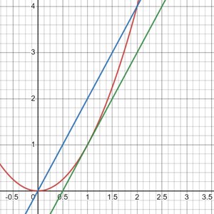
Additional info: The image above visually demonstrates the tangent (green) and secant (blue) lines to the curve y = x^2 at a point, reinforcing the concept of instantaneous versus average rate of change.

1.3 The Derivative and Limits

The derivative of a function at a point gives the slope of the tangent line, representing the instantaneous rate of change. For a function y = f(x), the derivative is denoted f'(x) or \frac{dy}{dx}.

• Derivative of a Linear Function: For y = mx + b, f'(x) = m.

• Derivative of a Constant: For y = c, f'(x) = 0.

• Power Rule: For f(x) = x^r,

• Geometric Meaning: f'(a) is the slope of the tangent to f(x) at x = a.

• Equation of Tangent Line:

• Difference Quotient: The average rate of change between x and x + h: As h → 0, this approaches the derivative.

1.4 Limits and the Derivative

Limits are fundamental to calculus, describing the behavior of functions as inputs approach a value. The derivative is defined as a limit.

• Definition of Limit: lim_{x→a} g(x) = L means g(x) approaches L as x approaches a.

• Limit Properties:

  • Sum:

  • Difference:

  • Product:

  • Quotient: (if denominator ≠ 0)

  • Constant Multiple:

  • Power:

• Derivative as a Limit:

• Limits at Infinity: Describes function behavior as x approaches infinity.

1.5 Differentiability and Continuity

A function is differentiable at a point if its derivative exists there. Differentiability implies continuity, but not vice versa. Common reasons for non-differentiability include discontinuities, corners, and vertical tangents.

• Continuity: A function is continuous at x = a if:

  1. f(a) is defined

  2. lim_{x→a} f(x) exists

  3. lim_{x→a} f(x) = f(a)

• Relationship: If f(x) is differentiable at x = a, then it is continuous at x = a.

1.6 Rules of Differentiation

Several rules simplify the process of finding derivatives:

• Constant Multiple Rule:

• Sum Rule:

• General Power Rule: For g(x) raised to a power r:

1.7 More about Derivatives

Derivatives can be taken with respect to any variable, and higher-order derivatives (such as the second derivative) provide information about the rate of change of the rate of change.

• Second Derivative:

• Notation: for the second derivative of y with respect to x.

• Applications: Second derivatives are used to analyze concavity and acceleration.

1.8 The Derivative as a Rate of Change

The derivative represents the instantaneous rate of change of a function. In business and science, this is used to model velocity, acceleration, marginal cost, and other rates.

• Average Rate of Change: Over interval [a, b]:

• Instantaneous Rate of Change: The derivative at a point.

• Velocity: If s(t) is position, then velocity is v(t) = s'(t).

• Acceleration: a(t) = v'(t) = s''(t).

• Marginal Cost/Revenue/Profit: The derivative of the cost, revenue, or profit function, representing the approximate change for producing one more unit.

Table: Summary of Limit Properties

Application Example: Slope as a Rate of Change

In the context of business, the slope of a graph at a point can represent the rate at which a resource (such as oil) is being used over time. The image below shows the calculation of the slope at a specific point, representing the rate of oil consumption.

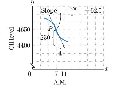
Additional info: The image above illustrates the physical significance of the slope at a point on a consumption graph, reinforcing the interpretation of the derivative as a rate of change in real-world business scenarios.