Ch. 3

Measures of Central Tendency

Definition and Overview

Measures of central tendency are statistical values that describe the center point or typical value of a dataset. The three main measures are the mean, median, and mode. These measures help summarize a large set of data with a single representative value.

• Mean: The arithmetic average, calculated by summing all values and dividing by the number of observations.

• Median: The middle value when data are arranged in order. If the number of observations is even, the median is the average of the two middle values.

• Mode: The value that appears most frequently in the dataset.

Calculating the Mean

The mean is calculated as follows:

Where are the data values and is the number of observations.

Example:

Calculate the mean for the data set: 87.2, 118.9, 76.2, 107.7, 61.5

Weighted Mean

The weighted mean assigns different weights to values, useful when some data points contribute more than others.

Where is the weight for each value .

Example:

Suppose exam, project, and homework scores are 94, 92, and 100, with weights 0.5, 0.35, and 0.15, respectively:

Median

The median is the value that divides the dataset into two equal halves. For an ordered dataset of size :

• If is odd, median is the value at position .

• If is even, median is the average of values at positions and .

Example:

Data: 70, 73, 74, 80, 82, 93, 95, 99 (n=8)

Median = (80 + 82)/2 = 81

Mode

The mode is the value with the highest frequency in the dataset. There can be no mode, one mode (unimodal), or multiple modes (bimodal, multimodal).

Example:

Data: 6, 7, 7, 8, 8, 8, 8, 8, 9, 9, 9, 10, 10, 11, 11, 11, 14, 14

Mode = 8 (appears 5 times)

Choosing the Appropriate Measure

Measures of Variation

Definition and Overview

Measures of variation describe the spread or dispersion of data values. Common measures include range, variance, standard deviation, and coefficient of variation.

• Range: Difference between the highest and lowest values.

• Variance: Average squared deviation from the mean.

• Standard Deviation: Square root of the variance, in the same units as the data.

• Coefficient of Variation (CV): Standard deviation as a percentage of the mean, useful for comparing variability between datasets with different units or means.

Range

Example:

Data: 10, 20, 30, 40, 50, 60, 70, 80, 90, 100

Range = 100 - 10 = 90

Variance and Standard Deviation

For a sample:

For a population:

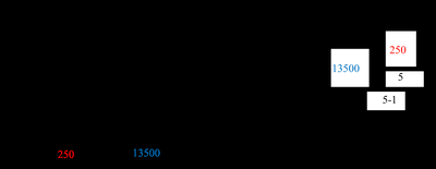
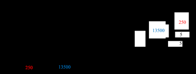
Coefficient of Variation (CV)

The coefficient of variation is calculated as:

Sample:

Population:

It allows comparison of variability between datasets with different units or means.

Using the Mean and Standard Deviation Together

Shapes of Frequency Distributions

Frequency distributions can be symmetric, left-skewed, or right-skewed. Skewness measures asymmetry, while kurtosis measures the peakedness of the distribution.

• Symmetric: Mean = Median

• Left-skewed: Mean < Median

• Right-skewed: Mean > Median

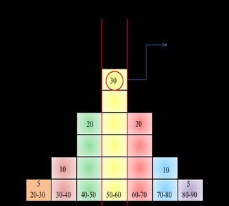
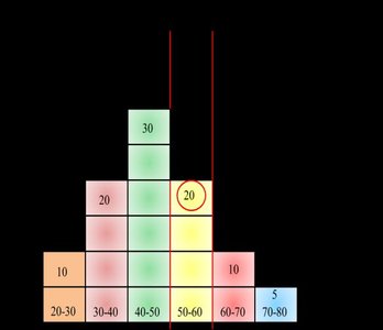
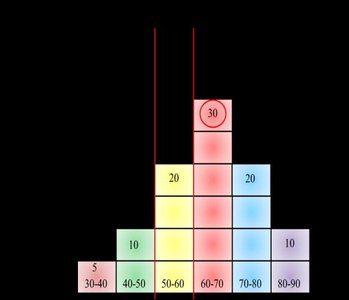
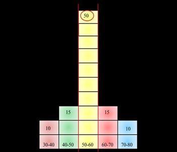
Quality Control Example

Histograms can illustrate how changes in mean and standard deviation affect the proportion of data within specification limits.

The z-Score

Definition and Calculation

The z-score indicates how many standard deviations a value is from the mean. It standardizes different datasets for comparison.

Population:

Sample:

Example:

Given , , :

The Empirical Rule and Chebyshev’s Theorem

The Empirical Rule

For bell-shaped (normal) distributions:

• ~68% of data within ±1 standard deviation

• ~95% within ±2 standard deviations

• ~99.7% within ±3 standard deviations

Chebyshev’s Theorem

For any distribution, at least of values fall within standard deviations of the mean, for .

Measures of Relative Position

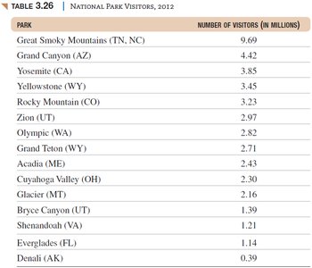
Percentiles and Quartiles

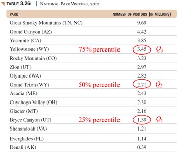
Percentiles divide data into 100 equal parts; quartiles divide data into four equal parts:

• Q1: 25th percentile

• Q2: 50th percentile (median)

• Q3: 75th percentile

Index for the pth percentile:

Example:

For 15 data points, the 70th percentile is at position (round up to 11th position).

Box-and-Whisker Plots

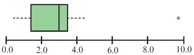
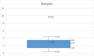
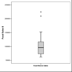
Boxplots display the five-number summary: minimum, Q1, median (Q2), Q3, and maximum. Outliers are values beyond or , where .

Descriptive Statistics in Excel

Using Excel for Descriptive Statistics

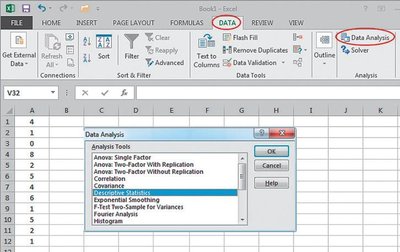
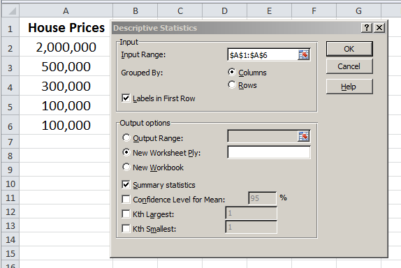
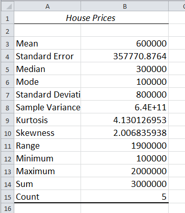
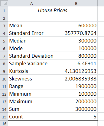
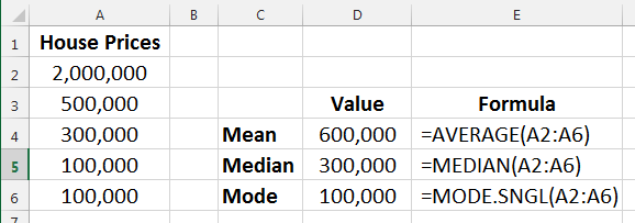
Excel provides tools for calculating mean, median, mode, standard deviation, variance, percentiles, and creating boxplots and histograms.

Application Examples

Music Downloads Example

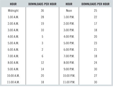
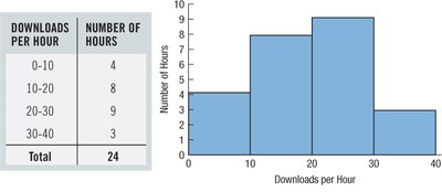
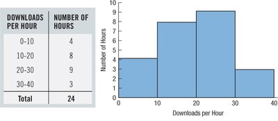
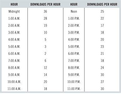
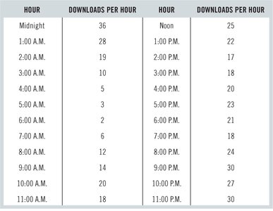
Given hourly download data, construct a histogram, calculate mean, median, range, quartiles, IQR, and standard deviation to summarize the distribution.

Food Store Sales Example

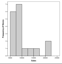
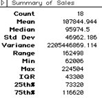
For a right-skewed distribution of store sales, the median is a better measure of central tendency than the mean, and the IQR is preferred over the standard deviation for measuring spread.

Ozone Levels Example

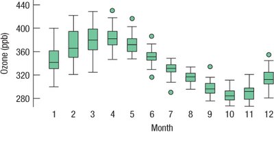
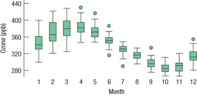
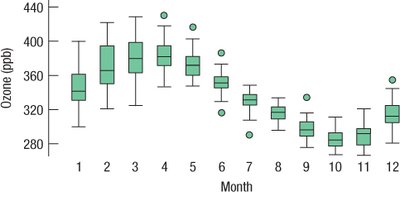
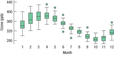
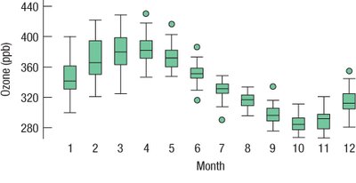
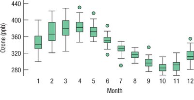
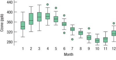
Boxplots can be used to compare distributions across months, identify months with highest values, largest IQR, and smallest range, and observe annual patterns.

Summary

• Central tendency: mean, median, mode

• Variation: range, variance, standard deviation, coefficient of variation

• Relative position: percentiles, quartiles, boxplots

• Excel can be used for all calculations and visualizations