Effect Sizes & Practical Significance

Introduction to Effect Sizes and Statistical Significance

Understanding the difference between statistical significance and practical (or clinical) significance is crucial in business statistics. Statistical tests help determine whether observed differences are likely due to chance, but effect sizes and confidence intervals provide context about the magnitude and importance of those differences.

Hypothesis Testing and ANOVA

Repeated Measures ANOVA Example

ANOVA (Analysis of Variance) is used to compare means across three or more groups. In a repeated measures design, the same subjects are measured under different conditions.

• Null Hypothesis (H0): All group means are equal.

• Alternative Hypothesis (HA): At least one group mean differs.

• Degrees of Freedom: Between groups: k-1; Within groups: (n-1)(k-1)

• Mean Squares: ,

• F-statistic:

• Decision Rule: Compare calculated F to critical value from F-table. If F < critical value, fail to reject H0.

Example: A pharmacist tests three routes of medication delivery in 12 patients. Calculated F = 1.59, critical F = 3.44 (α = 0.05). Since 1.59 < 3.44, there is insufficient evidence to conclude a difference in mean symptom relief.

Statistical Significance and p-values

Understanding p-values

A p-value is the probability of observing data as extreme as, or more extreme than, the sample result, assuming the null hypothesis is true. The conventional threshold for significance is α = 0.05.

• p < 0.05: Statistically significant; reject H0.

• p ≥ 0.05: Not statistically significant; fail to reject H0.

• Statistical significance does not imply practical importance.

Note: The difference between p = 0.049 and p = 0.051 is minimal in evidence, but the decision rule is binary.

Type I and Type II Errors

Definitions and Visualizations

Errors in hypothesis testing arise from the limitations of sampling.

• Type I Error (α): Rejecting H0 when it is true (false positive).

• Type II Error (β): Failing to reject H0 when it is false (false negative).

• Power: Probability of correctly rejecting a false H0 (1 - β). Conventionally, studies aim for power ≥ 0.80.

Multiple Comparisons Problem

Inflation of Type I Error

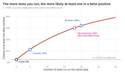
Conducting multiple statistical tests increases the chance of finding at least one significant result by chance (Type I error). Corrections such as Bonferroni or Tukey are used to control this risk.

• With 5 tests, the chance of at least one false positive is 23%.

• With 20 tests, the chance rises to 64%.

Effect Sizes

Definition and Importance

Effect size quantifies the magnitude of a difference or relationship, independent of sample size. It helps determine if a statistically significant result is meaningful in practice.

• Cohen's d (for t-tests): Small: 0.2, Medium: 0.5, Large: 0.8

• η² (eta-squared): Used for ANOVA.

• φ (phi), Cramér’s V: Used for chi-square tests.

Example: A large sample can make a tiny difference statistically significant, but the effect size reveals its practical importance.

Sample Size and Confidence Intervals

Sample Size Effects

Larger sample sizes yield more stable estimates and narrower confidence intervals (CIs). The standard error of the mean (SEM) decreases as sample size increases:

• To halve the CI width, sample size must be quadrupled.

Confidence Intervals (CIs) and Hypothesis Testing

Interpreting Confidence Intervals

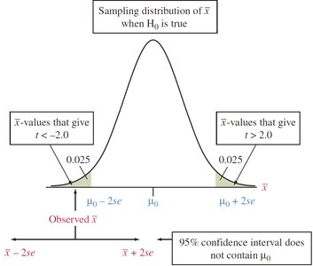
A 95% CI gives a range of plausible values for a population parameter. If the null value (e.g., mean difference = 0) is outside the CI, the result is statistically significant at α = 0.05.

• If the CI includes 0, the difference is not statistically significant.

• If the CI excludes 0, the difference is statistically significant.

Visualizing CI Overlap

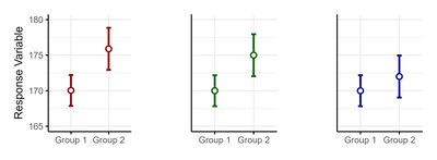
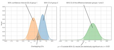
Comparing group means using CIs:

• Non-overlapping CIs suggest a significant difference.

• Overlapping CIs do not guarantee no significant difference; formal testing is required.

• Calculate the CI for the difference between means for robust inference.

Examples of Hypothesis Testing and CIs

Independent Samples t-test: BMI Example

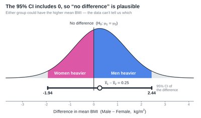
Comparing BMI between men and women (n = 41 each):

• t = 0.23, p > 0.05; fail to reject H0.

• 95% CI for mean difference: [-1.94, 2.44] (includes 0, so no significant difference).

One-Sample t-test: VO2max Example

Comparing current VO2max to historical value:

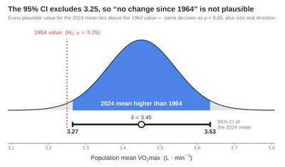
• Sample mean = 3.45, historical mean = 3.25, s = 0.65, n = 50

• t = 2.17 > 2.01 (critical), p < 0.05; reject H0.

• 95% CI: [3.27, 3.63] (does not include 3.25, so significant difference).

Two-Sample Proportions z-test: Aspirin Example

Comparing heart attack rates between aspirin and placebo groups:

• Placebo: 1.7%, Aspirin: 0.9%

• 95% CI for difference: [0.51%, 1.09%] (does not include 0, so significant difference).

Clinical vs. Statistical Significance

Minimal Clinically Important Difference (MCID)

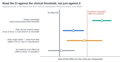
Statistical significance does not always imply clinical or practical importance. The MCID is the smallest change in an outcome that is meaningful to patients or practitioners.

• A result can be statistically significant but not clinically meaningful (e.g., tiny weight loss in a large sample).

• A result can be clinically meaningful but not statistically significant (e.g., large pain reduction in a small sample).

Chi-Square Goodness-of-Fit Test

Testing Categorical Distributions

The chi-square goodness-of-fit test compares observed frequencies in categories to expected frequencies under a specified distribution.

• Null Hypothesis (H0): The observed distribution matches the expected distribution.

• Test Statistic:

• Degrees of Freedom: df = k - 1 (k = number of categories)

• If calculated χ² > critical value, reject H0.

Conclusion: χ² = 21.43 > 5.99 (critical value, df = 2, α = 0.05), so the clinic's referrals do not match the national profile.