Ch 9

Hypothesis Testing: One-Sample Tests

Introduction to Hypothesis Testing

Hypothesis testing is a fundamental statistical method used to make inferences about population parameters based on sample data. It allows researchers to test claims about means, proportions, or variances by comparing observed sample statistics to theoretical values under the null hypothesis.

• Null Hypothesis (H0): Represents the status quo or a statement of no effect.

• Alternative Hypothesis (H1): Represents the claim or effect the researcher is testing for.

• Significance Level (α): The probability threshold for rejecting H0, commonly set at 0.01, 0.05, or 0.10.

• Test Statistic: A standardized value (z or t) calculated from sample data.

• Critical Value: The cutoff value that determines the rejection region for H0.

• P-value: The probability of observing a test statistic as extreme as, or more extreme than, the sample result, assuming H0 is true.

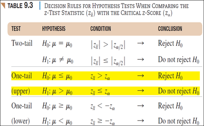
Decision Rules for Hypothesis Tests

Decision rules specify when to reject or not reject the null hypothesis based on the comparison between the test statistic and the critical value.

• Two-tailed test: Used when the alternative hypothesis is H1: μ ≠ μ0.

• One-tailed test (upper): Used when H1: μ > μ0.

• One-tailed test (lower): Used when H1: μ < μ0.

Hypothesis Test for Population Mean (σ Known)

When the population standard deviation (σ) is known, the z-test is used to test hypotheses about the population mean. The sampling distribution of the mean is assumed to be normal if n ≥ 30 (Central Limit Theorem) or if the population is normal.

• Test Statistic Formula:

• Critical Value: Determined from the standard normal (z) table based on α and tail type.

• Decision: Compare z to the critical value to decide whether to reject H0.

Hypothesis Test for Population Mean (σ Unknown)

When the population standard deviation is unknown, the t-test is used. The sample standard deviation (s) substitutes for σ, and the test statistic follows the Student's t-distribution with n-1 degrees of freedom.

• Test Statistic Formula:

• Critical Value: Determined from the t-distribution table based on α, tail type, and degrees of freedom.

• Decision: Compare t to the critical value to decide whether to reject H0.

Hypothesis Test for Population Proportion

Testing a population proportion uses the z-test, provided the sample size is large enough for the normal approximation (np ≥ 5 and n(1-p) ≥ 5).

• Test Statistic Formula:

• Critical Value: Determined from the standard normal (z) table.

• Decision: Compare z to the critical value to decide whether to reject H0.

Examples and Applications

Below are examples illustrating the application of hypothesis tests for means and proportions:

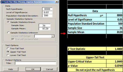
• Example 1 (Mean, σ Known): Testing if the average life of CFL bulbs exceeds 8,000 hours. Sample mean = 8,120, σ = 500, n = 36, α = 0.05. Calculated z = 1.44, critical value = 1.645. Since 1.44 < 1.645, do not reject H0.

• Example 2 (Mean, σ Unknown): Testing if the average cost of a hotel room in Chicago is less than $188. Sample mean = $177.50, s = $25.40, n = 25, α = 0.05. Calculated t = -2.07, critical value = -1.711. Since -2.07 < -1.711, reject H0.

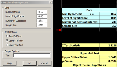
• Example 3 (Proportion): Testing if the proportion of cell phone users with 4G contracts has increased above 0.62. Sample proportion = 0.68, n = 350, α = 0.05. Calculated z = 2.31, critical value = 1.645. Since 2.31 > 1.645, reject H0.

Possible Outcomes and Errors in Hypothesis Testing

There are four possible outcomes in hypothesis testing, depending on the actual state of H0 and the decision made:

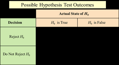
• Type I Error (α): Rejecting H0 when it is true.

• Type II Error (β): Failing to reject H0 when it is false.

Example: In quality control, Type I error is the producer's risk (finding a problem that does not exist), and Type II error is the consumer's risk (failing to detect a problem).

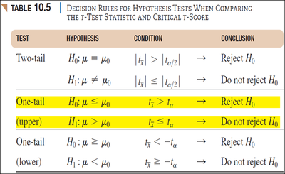
Summary Table: Hypothesis Test Decision Rules

The following tables summarize the decision rules for z-tests and t-tests:

Additional info:

These notes are expanded with academic context to ensure completeness and clarity for exam preparation. All formulas are provided in LaTeX format for mathematical rigor. Tables are recreated for comparison and classification purposes. Images included are directly relevant to the explanation of hypothesis testing decision rules and outcomes.