Chapter 5,6, and 7

Discrete and Continuous Probability Distributions

Overview of Probability Distributions

Probability distributions describe how probabilities are distributed over the values of a random variable. In business statistics, understanding the distinction between discrete and continuous probability distributions is essential for analyzing data and making informed decisions.

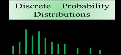
• Discrete Probability Distributions: Concern random variables that take on countable values (e.g., number of customers, number of defective items).

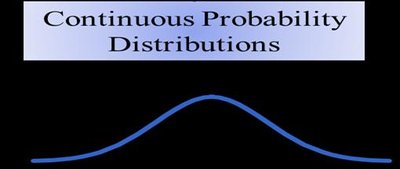
• Continuous Probability Distributions: Concern random variables that can take on any value within a given range (e.g., time, weight, temperature).

Discrete Probability Distributions

Definition and Properties

A discrete probability distribution lists all possible outcomes of a discrete random variable along with their associated probabilities. The probabilities must satisfy two conditions:

• Each probability is between 0 and 1, inclusive.

• The sum of all probabilities is 1:

Common types include the binomial, Poisson, and hypergeometric distributions.

Examples of Discrete Probability Distributions

• Number of heads in coin tosses

• Number of customers arriving at a store

• Number of defective products in a batch

For example, tossing two coins and counting the number of heads yields a probability distribution for 0, 1, or 2 heads.

Calculating Mean and Standard Deviation

The mean (expected value) and standard deviation of a discrete probability distribution are calculated as follows:

• Mean:

• Variance:

• Standard Deviation:

These measures provide insight into the central tendency and spread of the distribution.

Binomial Probability Distribution

Definition and Characteristics

The binomial distribution models the number of successes in a fixed number of independent trials, each with the same probability of success. The four requirements are:

• Fixed number of trials ()

• Each trial has two possible outcomes (success or failure)

• Trials are independent

• Probability of success () is constant for each trial

Binomial Probability Formula

The probability of exactly successes in trials is given by:

, where

The sum of probabilities for all possible values of (from 0 to ) equals 1.

Mean and Standard Deviation of Binomial Distribution

• Mean:

• Variance:

• Standard Deviation:

Example: Voters Supporting a Proposition

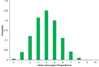
Suppose 40% of voters support a proposition. In a sample of 10 voters, the probability that exactly 5 support the proposition is:

Using Excel for Binomial Probabilities

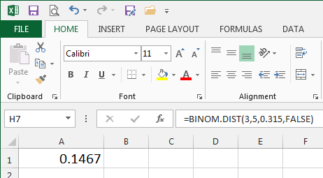
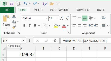
Excel provides the BINOM.DIST function to calculate binomial probabilities:

Syntax: =BINOM.DIST(x, n, p, cumulative)

• If cumulative is FALSE, it returns

• If cumulative is TRUE, it returns

Continuous Probability Distributions

Definition and Types

A continuous probability distribution describes the probabilities of the possible values of a continuous random variable. The probability that a continuous random variable equals any specific value is zero; instead, probabilities are assigned to intervals.

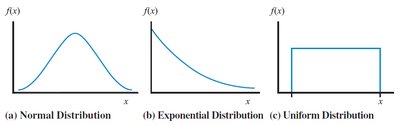
• Common types: Normal, Exponential, Uniform

Normal Probability Distribution

The normal distribution is a continuous, symmetric, bell-shaped distribution characterized by its mean () and standard deviation (). The probability density function is:

Key properties:

• Symmetric about the mean

• Total area under the curve is 1

• Mean = Median = Mode

Standard Normal Distribution and Z-Scores

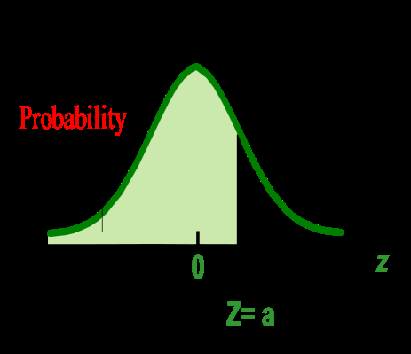
The standard normal distribution is a normal distribution with and . Any normal random variable can be converted to a standard normal variable using:

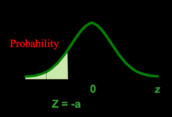
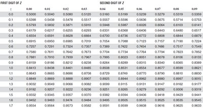
Calculating Probabilities Using Z-Tables

To find probabilities for normal distributions:

1. Draw a picture and shade the area of interest.

2. Convert values to scores.

3. Use the standard normal table to find the area (probability).

Excel Functions for Normal Probabilities

• NORM.DIST(x, mean, standard_dev, cumulative): Returns the probability for a normal distribution.

• NORM.S.DIST(z, cumulative): Returns the probability for the standard normal distribution.

Sampling Distributions and the Central Limit Theorem

Sampling Distribution of the Mean

The sampling distribution of the mean is the probability distribution of all possible sample means from samples of a given size drawn from a population. The mean of the sampling distribution is equal to the population mean (), and the standard deviation (standard error) is .

Central Limit Theorem (CLT)

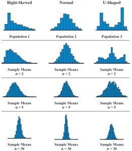
The Central Limit Theorem states that, for sufficiently large sample sizes (), the sampling distribution of the sample mean will be approximately normal, regardless of the population's distribution.

• As sample size increases, the sampling distribution becomes more normal and the standard error decreases.

Application of CLT in Hypothesis Testing

The CLT allows us to use normal probability methods to test claims about population means and proportions, even when the population distribution is not normal, provided the sample size is large enough.

Summary Table: Key Probability Distributions

Additional info: This guide covers the foundational probability distributions and their application in business statistics, including the use of Excel for calculations and the importance of the Central Limit Theorem for inferential statistics.