Applications of the Derivative

Maxima and Minima

The study of maxima and minima is fundamental in calculus, as it allows us to identify the highest and lowest values a function can attain within a given domain. These concepts are crucial for optimization and understanding the behavior of functions.

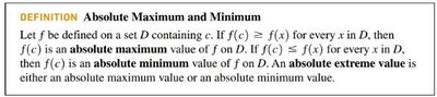
• Absolute Maximum: If $f(c) \geq f(x)$ for every $x$ in $D$, then $f(c)$ is an absolute maximum value of $f$ on $D$.

• Absolute Minimum: If $f(c) \leq f(x)$ for every $x$ in $D$, then $f(c)$ is an absolute minimum value of $f$ on $D$.

• Absolute Extreme Value: Either an absolute maximum or minimum value.

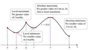
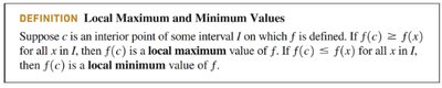
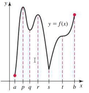
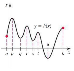
Local Maximum and Minimum: These are values that are the highest or lowest within a neighborhood of a point, not necessarily the entire domain.

• Local Maximum: $f(c) \geq f(x)$ for all $x$ in a neighborhood of $c$.

• Local Minimum: $f(c) \leq f(x)$ for all $x$ in a neighborhood of $c$.

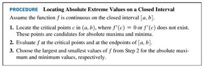
Locating Absolute Extreme Values on a Closed Interval

To find absolute maxima and minima on a closed interval, follow a systematic procedure:

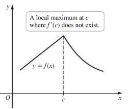
• Locate critical points where $f'(c) = 0$ or $f'(c)$ does not exist.

• Evaluate $f$ at critical points and endpoints.

• Choose the largest and smallest values for the absolute maximum and minimum, respectively.

Mean Value Theorem and Rolle's Theorem

Mean Value Theorem

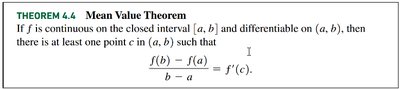
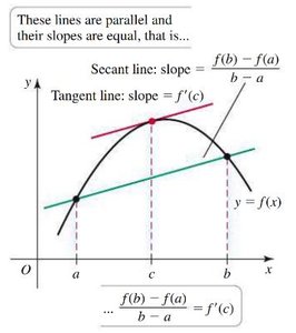
The Mean Value Theorem (MVT) is a fundamental result in calculus that connects the average rate of change of a function to its instantaneous rate of change.

• If $f$ is continuous on $[a, b]$ and differentiable on $(a, b)$, then there exists $c$ in $(a, b)$ such that:

$ \frac{f(b) - f(a)}{b - a} = f'(c) $

Rolle's Theorem

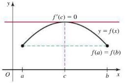
Rolle's Theorem is a special case of the Mean Value Theorem where the function has equal values at the endpoints.

• If $f(a) = f(b)$ and $f$ is continuous on $[a, b]$ and differentiable on $(a, b)$, then there exists $c$ in $(a, b)$ such that $f'(c) = 0$.

What Derivatives Tell Us: Increasing, Decreasing, and Concavity

Increasing and Decreasing Functions

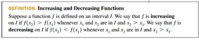
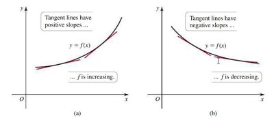
Derivatives provide information about whether a function is increasing or decreasing on an interval.

• Increasing: $f(x_2) > f(x_1)$ whenever $x_2 > x_1$.

• Decreasing: $f(x_2) < f(x_1)$ whenever $x_2 > x_1$.

Test for Intervals of Increase and Decrease

The sign of the first derivative determines whether a function is increasing or decreasing:

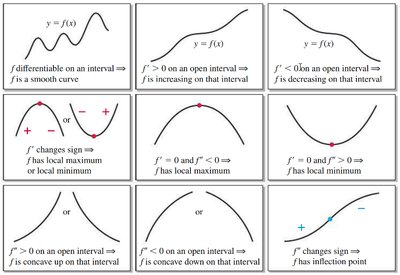
• If $f'(x) > 0$ on an interval, $f$ is increasing.

• If $f'(x) < 0$ on an interval, $f$ is decreasing.

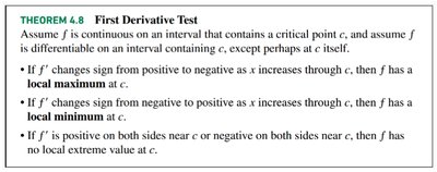
First Derivative Test

The First Derivative Test is used to classify critical points as local maxima or minima:

• If $f'$ changes from positive to negative at $c$, $f$ has a local maximum at $c$.

• If $f'$ changes from negative to positive at $c$, $f$ has a local minimum at $c$.

• If $f'$ does not change sign, $f$ has no local extreme value at $c$.

Concavity and Inflection Points

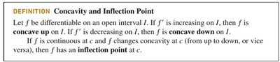
Concavity describes the direction in which a function curves. Inflection points are where the concavity changes.

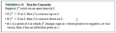
• Concave Up: $f'' > 0$ on an interval.

• Concave Down: $f'' < 0$ on an interval.

• Inflection Point: Where $f''$ changes sign.

Second Derivative Test for Local Extrema

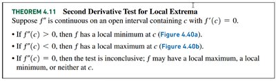
The Second Derivative Test provides a method to classify critical points:

• If $f''(c) > 0$, $f$ has a local minimum at $c$.

• If $f''(c) < 0$, $f$ has a local maximum at $c$.

• If $f''(c) = 0$, the test is inconclusive.

Graphing Functions

Graphing Guidelines

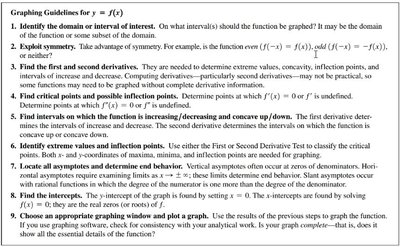
Graphing a function involves several steps to ensure all important features are captured:

• Identify the domain and interval of interest.

• Exploit symmetry.

• Find first and second derivatives.

• Find critical points and possible inflection points.

• Determine intervals of increase/decrease and concavity.

• Locate extreme values and inflection points.

• Locate all asymptotes and determine end behavior.

• Find intercepts.

• Sketch the graph.

Optimization Problems

Guidelines for Solving Applied Minimum and Maximum Problems

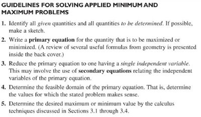
Optimization problems require finding the maximum or minimum value of a function subject to constraints.

• Identify all given and required quantities.

• Write a primary equation for the quantity to be optimized.

• Reduce to a single independent variable.

• Determine the feasible domain.

• Use calculus techniques to find the desired value.

Linear Approximation and Differentials

Linear Approximation

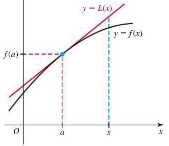
Linear approximation uses the tangent line at a point to estimate the value of a function near that point.

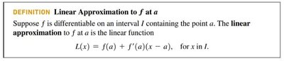
• The linear approximation to $f$ at $a$ is $L(x) = f(a) + f'(a)(x - a)$.

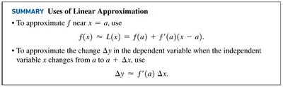
Uses of Linear Approximation

• To approximate $f$ near $x = a$, use $f(x) \approx L(x) = f(a) + f'(a)(x - a)$.

• To approximate the change $\Delta y$ when $x$ changes from $a$ to $a + \Delta x$, use $\Delta y \approx f'(a) \Delta x$.

Differentials

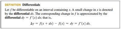
Differentials provide a way to approximate small changes in a function.

• A small change in $x$ is $dx$.

• The corresponding change in $f$ is $dy = f'(x) dx$.

• $\Delta y = f(x + dx) - f(x) \approx dy = f'(x) dx$.

Antiderivatives and Differential Equations

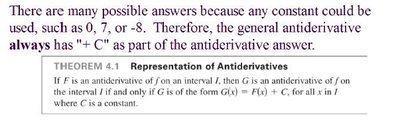
Antiderivative

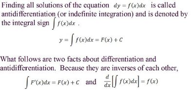
An antiderivative reverses the process of differentiation. It is also known as indefinite integration.

• A function $F$ is an antiderivative of $f$ if $F'(x) = f(x)$ for all $x$ in $I$.

• The general antiderivative includes a constant: $F(x) + C$.

Differential Equations

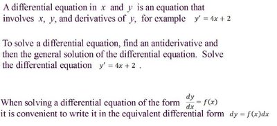
A differential equation involves derivatives of a function. Solving it requires finding an antiderivative.

• General solution: $y = \int f(x) dx = F(x) + C$.

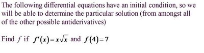
• Initial conditions allow determination of the particular solution.

Examples of Antiderivatives and Differential Equations

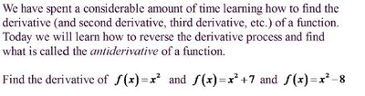
• Find the derivative and antiderivative of $f(x) = x^2$, $f(x) = x^2 + 7$, $f(x) = x^2 - 8$.

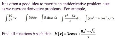
• Find all functions $h$ such that $h'(x) = 3 \cos x + \frac{8x^3 - \sqrt{x}}{x}$.

• Find $f$ if $F'(x) = x \sqrt{x}$ and $F(4) = 7$.

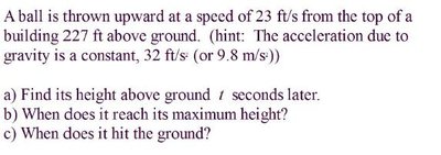
• Applied example: A ball is thrown upward; find its height, maximum height, and time to hit the ground.

Summary Table: Derivative and Integration Rules