Ch. 9 - Differential Equations
Briggs - Calculus: Early Transcendentals 3rd Edition
Briggs3rd EditionCalculus: Early TranscendentalsISBN: 9780136847243Non è quello che usi tu?Cambia libro di testo
Capitolo 9, Problema 9.R.19a

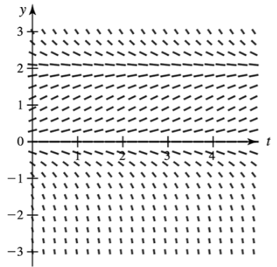
Direction fields Consider the direction field for the equation y′=y(2−y) shown in the figure and initial conditions of the form y(0)=A.
a. Sketch a solution on the direction field with the initial condition y(0)=1.
Direction field graph showing slope vectors for y′=y(2−y) with t-axis from 0 to 4 and y-axis from -3 to 3.

Guida verificata passo dopo passo
1
Identify the differential equation given: \(y' = y(2 - y)\). This tells us the slope of the solution curve at any point \((t, y)\) depends on the value of \(y\) at that point.
Note the initial condition \(y(0) = 1\). This means the solution curve must pass through the point \((0, 1)\) on the \(t\)-\(y\) plane.
Examine the direction field at \(y = 1\). Calculate the slope at this point using the differential equation: \(y' = 1 \times (2 - 1) = 1\). So, the slope of the solution curve at \(t=0\) and \(y=1\) is 1.
Using the slope from the direction field at \((0,1)\), sketch a curve starting at this point that follows the slope vectors shown in the direction field. The curve should move upward initially since the slope is positive.
Observe the behavior of the solution as \(t\) increases. Since \(y' = y(2 - y)\), when \(y\) approaches 2, the slope \(y'\) approaches zero, indicating the solution curve will level off near \(y=2\). Sketch the curve approaching this horizontal asymptote as \(t\) grows.

Risposta video verificata per un problema simile:

Questa soluzione video è stata consigliata dai nostri tutor come utile per risolvere questo problema.
Durata del video:
2m

Concetti chiave

Ecco i concetti essenziali che devi comprendere per rispondere correttamente alla domanda.

Direction Fields

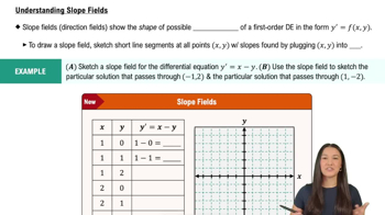
A direction field is a graphical representation of a first-order differential equation showing slope vectors at various points. Each small line segment indicates the slope of the solution curve passing through that point, helping visualize the behavior of solutions without solving the equation explicitly.
Video consigliato:
05:45
Understanding Slope Fields

Autonomous Differential Equations

An autonomous differential equation has the form y' = f(y), where the rate of change depends only on y, not on the independent variable t. This allows for analysis of equilibrium points and stability by examining where f(y) = 0, which correspond to constant solutions.
Video consigliato:
07:39
Classifying Differential Equations

Equilibrium Solutions and Stability

Equilibrium solutions occur where y' = 0, meaning the solution remains constant. Stability depends on the sign of the derivative of f(y) at these points: if small perturbations decay over time, the equilibrium is stable; if they grow, it is unstable. This helps predict long-term behavior of solutions.
Video consigliato:
04:00
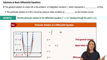
Solutions to Basic Differential Equations