Graphs and Functions

The Rectangular Coordinate System (Cartesian Plane)

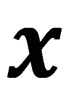
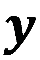
The rectangular coordinate system, also known as the Cartesian plane, is a two-dimensional plane formed by two perpendicular number lines: the horizontal x-axis and the vertical y-axis. This system is fundamental for graphing equations and visualizing relationships between variables in algebra.

• Axes: The x-axis is horizontal, and the y-axis is vertical. They intersect at the origin (0, 0).

• Ordered Pairs: Points are represented as (x, y), where x is the horizontal position and y is the vertical position.

• Quadrants: The axes divide the plane into four quadrants, numbered counterclockwise starting from the upper right.

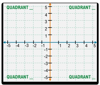
Example: The graph below shows the four quadrants of the coordinate plane.

Quadrant I: (+, +)    Quadrant II: (−, +)    Quadrant III: (−, −)    Quadrant IV: (+, −)

Plotting Points and Identifying Quadrants

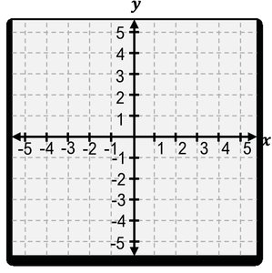
To plot a point, locate its x-value on the horizontal axis and its y-value on the vertical axis. The intersection is the location of the point.

• Example Points: A(4, 3), B(−3, 2), C(−2, −3), D(5, −4), E(0, 0), F(0, −3)

Each point lies in a specific quadrant or on an axis:

• Quadrant I: x > 0, y > 0

• Quadrant II: x < 0, y > 0

• Quadrant III: x < 0, y < 0

• Quadrant IV: x > 0, y < 0

• Points on axes: x = 0 or y = 0

Practice: Plotting and Identifying Points

Practice plotting points such as W(1, −2), X(5, 2), Y(−3, −4), Z(−4, 3) on the coordinate plane below.

Determining If an Ordered Pair Is a Solution

An ordered pair (x, y) is a solution to a two-variable equation if substituting x and y into the equation makes it true.

• One-variable equation: x + 2 = 5 → x = 3 is a solution because 3 + 2 = 5.

• Two-variable equation: x + 2y = 5. (3, 1) is a solution because 3 + 2(1) = 5.

Example: Which of the following are solutions to x + 2y = 5?

• (5, 0): 5 + 2(0) = 5 ✓

• (8, 2): 8 + 2(2) = 12 ✗

• (−3, 4): −3 + 2(4) = 5 ✓

Completing Ordered Pair Solutions

To complete an ordered pair solution for an equation, substitute the given value and solve for the missing variable.

• Example: For y = 2x + 3, if x = 2, then y = 2(2) + 3 = 7, so (2, 7) is a solution.

• If y = 5, then 5 = 2x + 3 → x = 1, so (1, 5) is a solution.

Graphing Linear Equations in Two Variables

The graph of a linear equation in two variables is a straight line. To graph:

1. Find ordered pair solutions by plugging in x-values to find y-values.

2. Plot the points and connect them with a straight line.

Example: Graph y = 4x − 3 by plotting points for several x-values and connecting them.

Intro to Relations and Functions

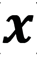
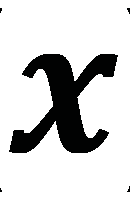
A relation is a set of ordered pairs (x, y). A function is a relation where each input (x) is paired with at most one output (y).

• Relations can be represented as sets, tables, graphs, or equations.

• Functions pass the vertical line test: any vertical line crosses the graph at most once.

Domain and Range

The domain of a relation or function is the set of all possible x-values (inputs). The range is the set of all possible y-values (outputs).

• Write the domain and range as lists or using interval notation.

• Example: For the set {(−4, 2), (−3, −5), (3, 4), (5, −2)}, the domain is {−4, −3, 3, 5} and the range is {2, −5, 4, −2}.

Function Notation

If an equation is a function, it can be written as y = f(x), read as "f of x." This notation emphasizes the dependence of y on x.

• Example: If f(x) = 3x − 1, then f(4) = 3(4) − 1 = 11.

Graphing Linear Equations Using Intercepts

The x-intercept is where the graph crosses the x-axis (y = 0). The y-intercept is where the graph crosses the y-axis (x = 0).

• To find the x-intercept, set y = 0 and solve for x.

• To find the y-intercept, set x = 0 and solve for y.

Slope of a Line

The slope (m) of a line measures its steepness and is calculated as the change in y divided by the change in x between two points:

$m = \frac{y_2 - y_1}{x_2 - x_1}$

• Types of Slope: Positive (line rises), Negative (line falls), Zero (horizontal), Undefined (vertical).

Slope-Intercept Form

The slope-intercept form of a line is $y = mx + b$, where m is the slope and b is the y-intercept.

• Example: For y = 2x + 3, the slope is 2 and the y-intercept is 3.

Parallel and Perpendicular Lines

• Parallel lines have the same slope but different y-intercepts.

• Perpendicular lines have slopes that are negative reciprocals of each other (e.g., m and −1/m).

Point-Slope Form

The point-slope form of a line is $y - y_1 = m(x - x_1)$, where (x₁, y₁) is a point on the line and m is the slope.

• Convert to slope-intercept form by solving for y.

Linear Inequalities in Two Variables

A linear inequality in two variables divides the plane into a region of solutions. The boundary is a line, which is solid for ≤ or ≥ and dashed for < or >.

• To graph, first draw the boundary line, then shade the region that satisfies the inequality.

• Test a point (often the origin) to determine which side to shade.

Example: Graph y > 2x − 4. Draw the line y = 2x − 4 (dashed), then shade above the line.

*Additional info: This summary covers the main concepts, definitions, and procedures for graphing and analyzing linear equations, relations, and functions as presented in the provided materials. Practice problems and examples are included to reinforce understanding.*