Consumer Behavior

The Buyer's Problem

Consumer behavior in microeconomics is centered around the buyer's problem, which consists of three main components: preferences, prices, and budget. Understanding these elements helps explain how consumers make choices to maximize their well-being.

• Preferences: Consumers have unique tastes and preferences, but are assumed to be rational and seek to maximize their satisfaction given constraints.

• Prices: Prices are taken as fixed, and consumers can purchase any quantity without affecting the market price.

• Budget: Consumers face a budget constraint, which limits their spending to available income.

Demand Curve and Marginal Decision-Making

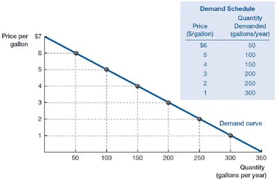
The demand curve reflects the relationship between the price of a good and the quantity demanded. Consumers make decisions at the margin, weighing the additional benefit of consuming one more unit against its cost.

• Individual Demand Curve: Shows willingness and ability to pay for each unit.

• Marginal Benefit: The extra benefit from consuming one more unit.

• Marginal Cost: The extra cost incurred from consuming one more unit.

Budget Constraints

Budget Set and Constraint

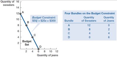
The budget constraint represents all possible combinations of goods a consumer can purchase given their income and the prices of goods. The slope of the budget line reflects the opportunity cost of one good in terms of another.

• Budget Equation: $50j + 25s = 300$ (where j = jeans, s = sweaters)

• Opportunity Cost: The number of units of one good forgone to obtain an additional unit of another good.

• Purchasing Whole Units: Consumers buy whole units, not fractions.

Graphing the Budget Set

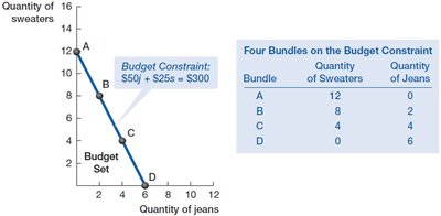
Graphically, the budget set is the area under the budget line, representing all affordable combinations. The slope is determined by the ratio of prices.

• Slope of Budget Line: $-\frac{P_j}{P_s}$

• General Form: $Q_y = \frac{B}{P_y} - \frac{P_x}{P_y} Q_x$

Opportunity Cost

Opportunity cost is a fundamental concept in economics, representing the value of the next best alternative forgone.

• Opportunity Cost of Jeans: $\frac{\text{Loss in sweaters}}{\text{Gain in jeans}} = \frac{P_j}{P_s}$

• Opportunity Cost of Sweaters: $\frac{\text{Loss in jeans}}{\text{Gain in sweaters}} = \frac{P_s}{P_j}$

Optimization and Consumer Equilibrium

Maximizing Net Benefit

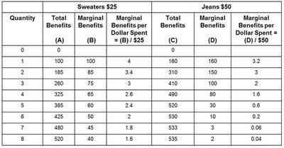
Consumers maximize their net benefit by equating the marginal benefit per dollar spent across all goods, subject to their budget constraint.

• Equilibrium Condition: $\frac{MB_s}{P_s} = \frac{MB_j}{P_j}$

• Budget Constraint: $s \cdot P_s + j \cdot P_j = 300$

Benefits and Costs Table

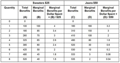
Tables of total and marginal benefits help illustrate how consumers decide the optimal quantity of each good to purchase.

Price and Income Changes

Effects of Price Changes

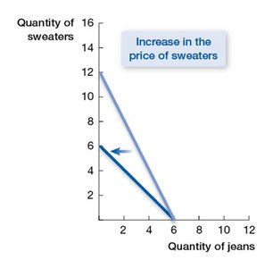
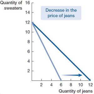
Changes in the price of goods pivot the budget constraint, altering the set of affordable combinations. An increase in price pivots the budget line inward, while a decrease pivots it outward.

• Inward Pivot: Price increase reduces affordable quantity.

• Outward Pivot: Price decrease increases affordable quantity.

Effects of Income Changes

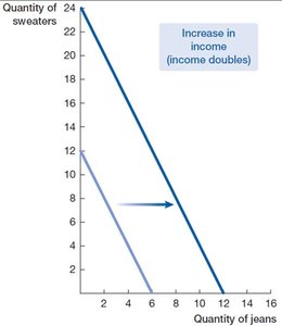
An increase in income shifts the budget constraint outward, allowing the consumer to purchase more of both goods.

• Outward Shift: More income increases the set of affordable bundles.

Consumer Surplus

Definition and Calculation

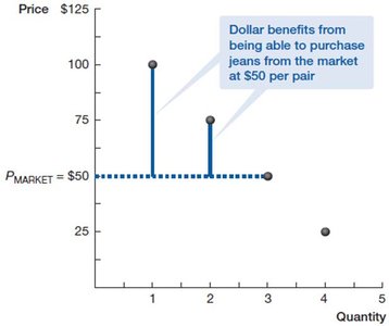
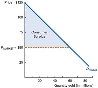
Consumer surplus is the difference between what a buyer is willing to pay and what they actually pay. It is a measure of changes in well-being and is often represented as the area between the demand curve and the market price.

• Consumer Surplus Formula: $\text{Consumer Surplus} = \frac{1}{2} \times \text{Base} \times \text{Height}$

• Market-Wide Surplus: Sum of individual surpluses across all buyers.

Preferences and Utility Functions

Utility Functions and Rational Preferences

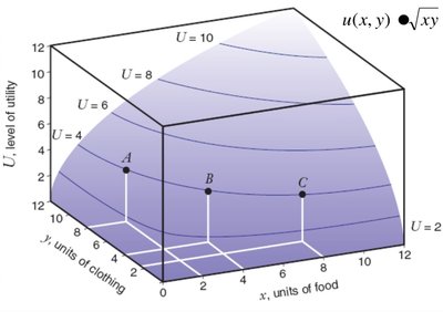
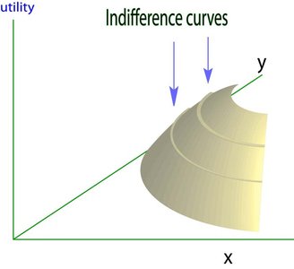
Utility functions mathematically represent consumer preferences, assuming completeness and transitivity. Indifference curves illustrate combinations of goods that yield the same utility.

• Utility Function: $U = f(x, y)$

• Indifference Curve: Shows all combinations of goods with equal utility.

• Marginal Rate of Substitution (MRS): $\frac{MU_x}{MU_y}$, the slope of the indifference curve.

Elasticity

Price Elasticity of Demand

Elasticity measures the responsiveness of one variable to changes in another. Price elasticity of demand quantifies how much quantity demanded changes in response to price changes.

• Formula: $E_D = \frac{\%\Delta Q}{\%\Delta P}$

• Interpretation: Elastic ($E_D > 1$), Inelastic ($E_D < 1$), Unit Elastic ($E_D = 1$)

Arc Elasticity

Arc elasticity uses average values to calculate elasticity between two points, providing a stable measure regardless of direction.

• Formula: $E_D = \frac{\Delta Q / (Q_1 + Q_2)/2}{\Delta P / (P_1 + P_2)/2}$

Cross-Price and Income Elasticity

Cross-price elasticity measures how the quantity demanded of one good changes with the price of another. Income elasticity measures how quantity demanded changes with income.

• Cross-Price Elasticity: $E_{CP} = \frac{\%\Delta Q_1}{\%\Delta P_2}$

• Income Elasticity: $E_I = \frac{\%\Delta Q}{\%\Delta I}$

• Interpretation: Negative (complements), Zero (independent), Positive (substitutes); Inferior, Normal, Luxury goods.

Determinants of Elasticity

Factors Affecting Price Elasticity

Several factors determine the price elasticity of demand, including the availability of substitutes, the share of the budget spent on the good, and the time horizon for adjustment.

• Substitutes: More substitutes increase elasticity.

• Budget Share: Higher share increases elasticity.

• Time Horizon: Longer horizons increase elasticity.

Applications and Examples

Consumer Choice and Surplus

Examples and tables illustrate how consumers optimize their choices and how changes in price and income affect their well-being and market outcomes.

• Example: Budget constraint for jeans and sweaters, calculation of consumer surplus, and elasticity measures.

Summary Table: Elasticity Types

Additional info: Academic context and formulas have been expanded for clarity and completeness. Only directly relevant images and tables have been included to reinforce key concepts.