Concepts of Motion

Introduction to Motion

Understanding motion is fundamental to physics. Motion describes the change in position of an object over time and can be classified into several basic types. This chapter introduces the foundational concepts and representations used to analyze motion in physics.

Types of Motion

• Linear Motion: Movement along a straight path.

• Circular Motion: Movement along a circular path.

• Projectile Motion: Curved path under the influence of gravity.

• Rotational Motion: Spinning around an axis.

Representing Motion

Motion Diagrams

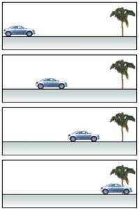
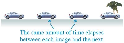
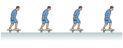
A motion diagram is a visual tool that shows an object's position at successive times. By analyzing these diagrams, we can infer whether an object moves at constant speed, speeds up, or slows down.

• Each frame in a motion diagram represents the object's position at a specific instant.

• Equally spaced images indicate constant speed.

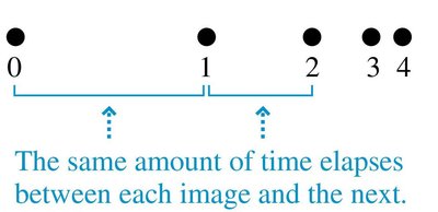
• Increasing distance between images shows speeding up; decreasing distance shows slowing down.

The Particle Model

In many cases, we simplify an object to a particle—treating all its mass as concentrated at a single point. This model is useful for analyzing motion without considering the object's size or shape.

• Each dot in a motion diagram represents the object's position as a particle.

Position, Displacement, and Vectors

Position and Coordinate Systems

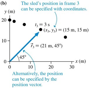
To describe motion quantitatively, we use a coordinate system. The position of an object is its location relative to an origin, often specified by coordinates (x, y).

Displacement

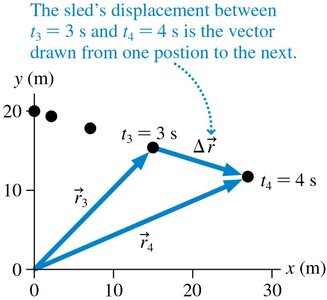
Displacement is a vector that represents the change in position of an object. It is drawn as an arrow from the initial to the final position.

• Symbol:

• Formula:

Vector Addition and Subtraction

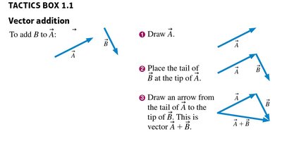
Vectors are added graphically by placing the tail of one at the tip of another. The resultant vector is drawn from the tail of the first to the tip of the last.

• To add vectors and : Place the tail of at the tip of , then draw the resultant.

• To subtract vectors: Reverse the direction of the vector to be subtracted and then add.

Time, Speed, and Velocity

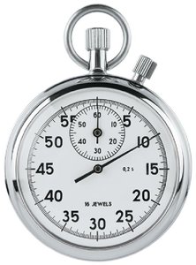
Time Interval

The time interval is the difference between the final and initial times: .

Average Speed and Average Velocity

• Average speed is the total distance traveled divided by the time interval:

• Average velocity is the displacement divided by the time interval:

Velocity Vectors in Motion Diagrams

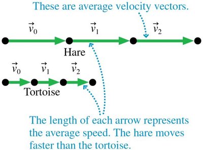
Velocity vectors are drawn in the direction of motion, with length proportional to speed. They connect successive positions in a motion diagram.

Acceleration

Linear Acceleration

Acceleration describes the rate of change of velocity. It is a vector quantity.

• Change in velocity:

• Average acceleration:

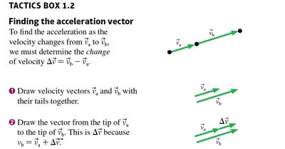
Finding the Acceleration Vector

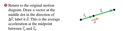
To find the acceleration vector, determine the change in velocity between two points and divide by the time interval. The acceleration vector is drawn at the midpoint between the two velocity vectors.

Speeding Up or Slowing Down

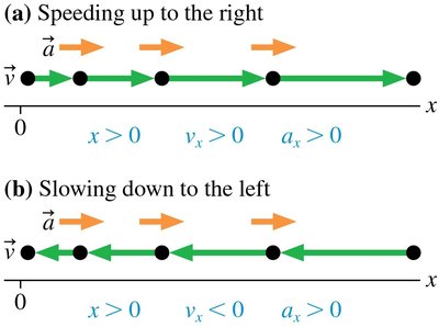
• If acceleration and velocity vectors point in the same direction, the object speeds up.

• If they point in opposite directions, the object slows down.

• Constant velocity occurs only when acceleration is zero.

Graphical Representation of Motion

Position-versus-Time Graphs

Another way to represent motion is with a graph of position (x) versus time (t). The slope of the graph at any point gives the velocity.

Problem-Solving in Physics

Representations in Problem Solving

• Verbal: Problem statement in words.

• Pictorial: Diagrams, motion diagrams, and coordinate systems.

• Graphical: Graphs of variables such as x vs. t.

• Mathematical: Equations relating physical quantities.

General Problem-Solving Strategy

1. Model: Simplify the situation using an appropriate model (e.g., particle model).

2. Visualize: Draw diagrams and graphs to clarify the problem.

3. Solve: Develop and solve equations using defined symbols.

4. Review: Check units, reasonableness, and consistency of the result.

Units and Measurement

SI Units

• Time: second (s)

• Length: meter (m)

• Mass: kilogram (kg)

Prefixes are used to denote powers of ten (e.g., kilo-, centi-, milli-).

Unit Conversions

Unit conversions are performed using ratios equal to one. For example, to convert feet to meters:

Significant Figures and Estimation

Significant Figures

• The number of significant figures reflects the precision of a measurement.

• When multiplying or dividing, the result should have as many significant figures as the least precise input.

• When adding or subtracting, the result should have the same number of decimal places as the least precise input.

Orders of Magnitude and Estimating

An order-of-magnitude estimate is a rough approximation, usually to one significant figure, denoted by the symbol ~ (e.g., mph).

Summary Table: Key Quantities and Their SI Units

Additional info: This summary includes expanded academic context and examples to ensure the notes are self-contained and suitable for exam preparation.