Kinematics in Two Dimensions

Introduction to Motion in a Plane

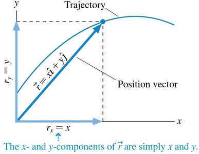
Motion in two dimensions involves the study of objects moving along paths in the x-y plane, such as projectiles or particles following curved trajectories. Unlike one-dimensional motion, two-dimensional kinematics requires the use of vectors to describe position, velocity, and acceleration.

• Position Vector (\(\vec{r}\)): Locates a particle in the plane using x and y components.

• Trajectory: The actual path followed by the particle, not just an abstract representation.

• Graphs: Typically plot y versus x to visualize motion.

Displacement and Velocity in Two Dimensions

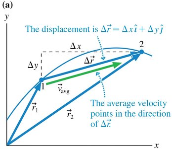
Displacement and velocity are vector quantities in two-dimensional motion. The displacement vector \(\Delta \vec{r}\) points from the initial to the final position, and the average velocity is the displacement divided by the time interval.

• Displacement: \(\Delta \vec{r} = \Delta x \hat{i} + \Delta y \hat{j}\)

• Average Velocity: \(\vec{v}_{avg} = \frac{\Delta \vec{r}}{\Delta t} = \frac{\Delta x}{\Delta t} \hat{i} + \frac{\Delta y}{\Delta t} \hat{j}\)

Instantaneous Velocity

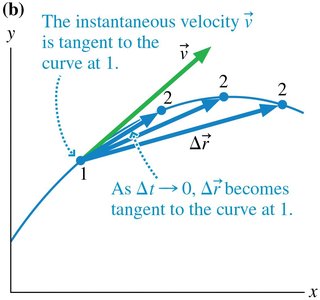
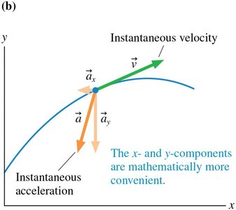
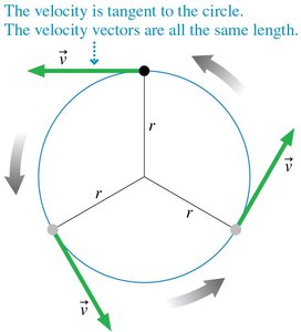
The instantaneous velocity is the limit of the average velocity as the time interval approaches zero. It is always tangent to the trajectory at any point.

• Instantaneous Velocity: \(\vec{v} = \lim_{\Delta t \to 0} \frac{\Delta \vec{r}}{\Delta t} = \frac{d\vec{r}}{dt} = \frac{dx}{dt} \hat{i} + \frac{dy}{dt} \hat{j}\)

• Component Form: \(\vec{v} = v_x \hat{i} + v_y \hat{j}\), where \(v_x = \frac{dx}{dt}\) and \(v_y = \frac{dy}{dt}\)

Velocity Components and Direction

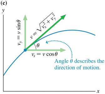
The velocity vector can be decomposed into x and y components using trigonometric functions. The speed is the magnitude of the velocity vector, and the direction is given by the angle \(\theta\) from the positive x-axis.

• Velocity Components:

  • \(v_x = v \cos \theta\)

  • \(v_y = v \sin \theta\)

• Speed: \(v = \sqrt{v_x^2 + v_y^2}\)

• Direction: \(\theta = \tan^{-1} \left(\frac{v_y}{v_x}\right)\)

Acceleration in Two Dimensions

Average and Instantaneous Acceleration

Acceleration is the rate of change of velocity. The average acceleration vector points in the direction of the change in velocity, and instantaneous acceleration is the limit as the time interval approaches zero.

• Average Acceleration: \(\vec{a}_{avg} = \frac{\Delta \vec{v}}{\Delta t}\)

• Instantaneous Acceleration: \(\vec{a} = \frac{d\vec{v}}{dt}\)

• Velocity can change in magnitude (speed) or direction.

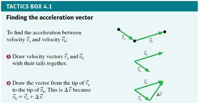
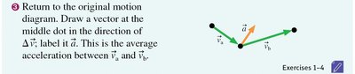
Decomposing Acceleration

Acceleration can be decomposed into components parallel and perpendicular to the velocity vector. The parallel component changes speed, while the perpendicular component changes direction.

• Parallel Component (\(\vec{a}_{\parallel}\)): Changes the speed of the object.

• Perpendicular Component (\(\vec{a}_{\perp}\)): Changes the direction of motion.

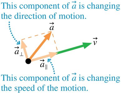
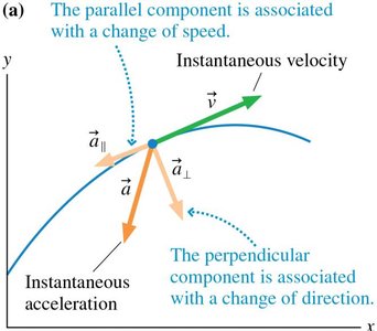
Mathematical Decomposition

Acceleration can also be decomposed into x and y components, which are mathematically convenient for calculations.

• \(a_x = \frac{dv_x}{dt}\)

• \(a_y = \frac{dv_y}{dt}\)

Constant Acceleration

If acceleration is constant, the kinematic equations for each component apply independently, but the time interval \(\Delta t\) is the same for both x and y directions.

• \(x_f = x_i + v_{ix} \Delta t + \frac{1}{2} a_x (\Delta t)^2\)

• \(y_f = y_i + v_{iy} \Delta t + \frac{1}{2} a_y (\Delta t)^2\)

• \(v_{fx} = v_{ix} + a_x \Delta t\)

• \(v_{fy} = v_{iy} + a_y \Delta t\)

Projectile Motion

Definition and Characteristics

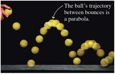
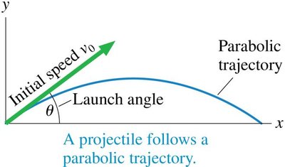
Projectile motion describes the motion of an object moving in two dimensions under the influence of gravity alone, neglecting air resistance. The trajectory is always a parabola.

• Projectile: Any object launched into the air and subject only to gravity.

• Trajectory: Parabolic path.

• Horizontal and Vertical Components: Treated independently.

Initial Velocity and Launch Angle

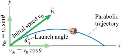
The initial velocity vector can be broken into horizontal and vertical components using the launch angle \(\theta\).

• \(v_{0x} = v_0 \cos \theta\)

• \(v_{0y} = v_0 \sin \theta\)

Acceleration in Projectile Motion

Gravity acts downward, so the vertical acceleration is \(-g\), while the horizontal acceleration is zero.

• \(a_x = 0\)

• \(a_y = -g\)

Projectile Motion Example

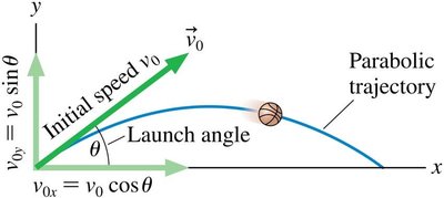
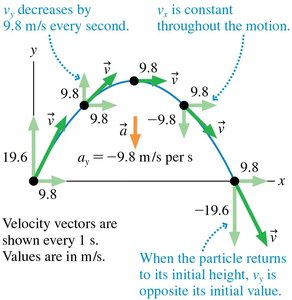
For a projectile launched from the origin with \(\vec{v}_0 = (9.8 \hat{i} + 19.6 \hat{j})\) m/s, the horizontal velocity remains constant, while the vertical velocity decreases by 9.8 m/s every second due to gravity.

Solving Projectile Motion Problems

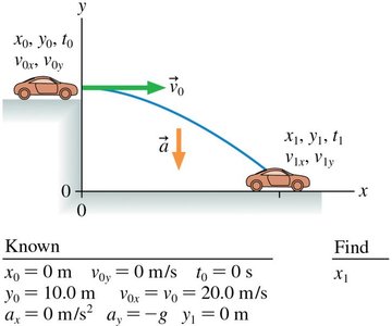
Projectile motion problems require separating the motion into horizontal and vertical components, using the same time interval for both.

• Horizontal: \(x_1 = x_0 + v_{0x} t_1\)

• Vertical: \(y_1 = y_0 + v_{0y} t_1 - \frac{1}{2} g t_1^2\)

• Find time from the vertical equation, then use it in the horizontal equation.

Independence of Horizontal and Vertical Motion

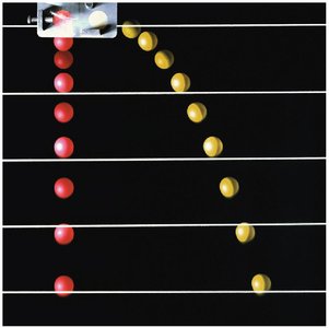
The horizontal and vertical motions of a projectile are independent. For example, a ball launched horizontally and a ball dropped from the same height will hit the ground simultaneously if air resistance is neglected.

Gravity's Effect on Trajectory

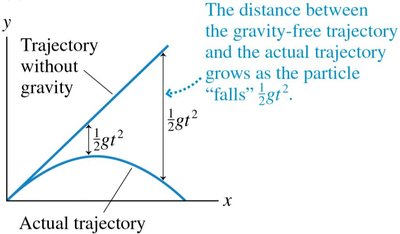
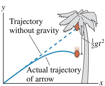
Gravity causes a projectile to fall below the straight-line path it would follow without gravity. The separation grows as \(\frac{1}{2} g t^2\), giving the trajectory its parabolic shape.

Summary of Projectile Motion Equations

• \(x_f = x_i + v_{ix} \Delta t\)

• \(y_f = y_i + v_{iy} \Delta t - \frac{1}{2} g (\Delta t)^2\)

• \(v_{fx} = v_{ix} = \text{constant}\)

• \(v_{fy} = v_{iy} - g \Delta t\)

Circular Motion

Introduction to Circular Motion

Circular motion is a special case of two-dimensional motion where an object moves along a circular path. Examples include a ball on a roulette wheel, satellites in orbit, or a ball on a string.

Uniform Circular Motion

Uniform circular motion occurs when a particle moves at constant speed around a circle of radius r. The period T is the time to complete one revolution, and the speed is given by:

• \(v = \frac{2\pi r}{T}\)

Angular Position and Arc Length

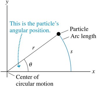
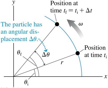
The angular position \(\theta\) is measured from the positive x-axis. If measured in radians, the arc length s is related to \(\theta\) by:

• \(s = r \theta\) (with \(\theta\) in radians)

Angular Velocity

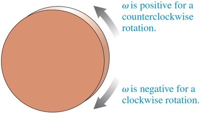
Angular velocity \(\omega\) is the rate at which the angular position changes. It can be positive or negative depending on the direction of rotation.

• \(\omega = \frac{d\theta}{dt}\)

• \(\omega = \frac{2\pi}{T}\) for uniform circular motion

Graphical Representation of Angular Velocity

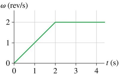
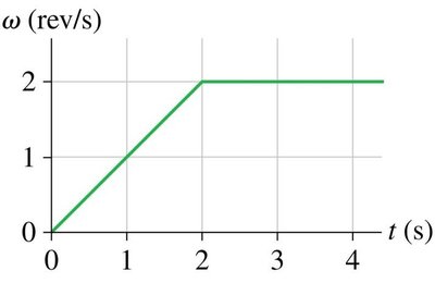
The slope of a \(\theta\) versus t graph gives \(\omega\), and the area under an \(\omega\) versus t curve gives the angular displacement.

Tangential Velocity

The tangential velocity \(v_t\) is the rate at which the particle moves around the circle, related to angular velocity by:

• \(v_t = \omega r\)

Centripetal Acceleration

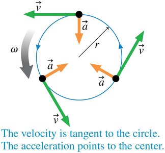
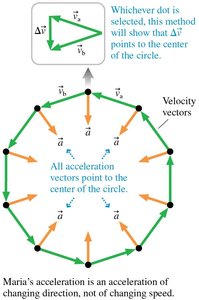
In uniform circular motion, the velocity vector changes direction, resulting in centripetal acceleration directed toward the center of the circle. The magnitude is:

• \(a = \frac{v^2}{r} = \omega^2 r\)

Example: Ferris Wheel

For a Ferris wheel of radius 9.0 m rotating 2.0 times per minute, the speed and acceleration of a rider are:

• Period: \(T = 30\) s

• Speed: \(v_t = \frac{2\pi r}{T} = 1.88\) m/s

• Centripetal acceleration: \(a = \frac{v_t^2}{r} = 0.39\) m/s2

Summary Table: Key Equations in Two-Dimensional Kinematics

Additional info: These notes expand on the original slides and images, providing full academic context, definitions, and examples for each concept. All equations are formatted in LaTeX for clarity and exam preparation.