Motion Along a Straight Line

Displacement and Position Vectors

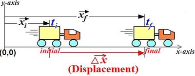
In kinematics, the position vector \( \vec{x} \) describes the location of an object along a straight line, typically referenced from an origin. The initial position is denoted as \( \vec{x}_i \) and the final position as \( \vec{x}_f \). The displacement is the change in position and is a vector quantity, meaning it has both magnitude and direction.

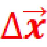
• Displacement Formula: The displacement \( \Delta \vec{x} \) is given by the difference between the final and initial position vectors:

• Example: If a truck moves from \( \vec{x}_i = 0 \) m to \( \vec{x}_f = 50 \) m, the displacement is \( 50 \) m in the positive x-direction.

Distance vs. Displacement

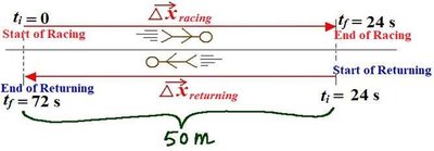
Distance is a scalar quantity representing the total length of the path traveled, regardless of direction. Displacement is a vector and only considers the straight-line change from the initial to the final position.

• Key Difference: Distance is always positive; displacement can be positive, negative, or zero.

• Example: If a runner goes 50 m forward and returns 50 m back to the start, the distance is 100 m, but the displacement is 0 m.

Average Velocity and Average Speed

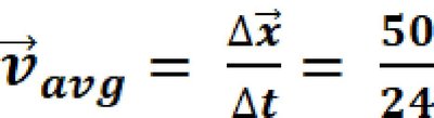
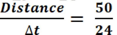
Average velocity is defined as the displacement divided by the time interval. It is a vector quantity and can be positive, negative, or zero. Average speed is the total distance traveled divided by the time interval and is always positive.

• Average Velocity Formula:

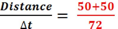
• Average Speed Formula:

• Example: If a person travels 50 m in 24 s, the average velocity is \( \frac{50}{24} \) m/s in the direction of motion.

• Round Trip Example: If the person returns to the starting point in another 24 s, the total displacement is 0, so average velocity is 0, but average speed is \( \frac{100}{48} \) m/s.

Position-Time and Velocity-Time Graphs

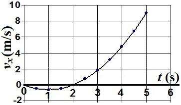
Graphs are essential tools for visualizing motion. A position-time graph shows how position changes with time, while a velocity-time graph shows how velocity changes with time.

• Position-Time Graph: The slope at any point gives the instantaneous velocity.

• Velocity-Time Graph: The slope gives the acceleration, and the area under the curve gives the displacement.

Acceleration

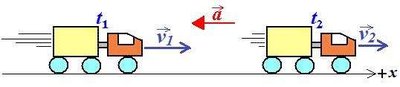
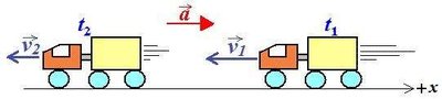
Acceleration is the rate of change of velocity with respect to time. It is a vector quantity and can be positive (speeding up) or negative (slowing down, also called deceleration).

• Formula:

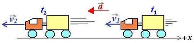
• Example: If a truck changes its velocity from \( \vec{v}_1 \) to \( \vec{v}_2 \) over a time interval, the acceleration vector points in the direction of the change.

Equations of Motion for Constant Acceleration

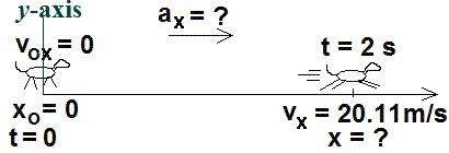
When acceleration is constant, the following kinematic equations describe the motion:

These equations allow us to solve for unknowns such as position, velocity, or time when the other quantities are known.

Relative Motion and Multiple Objects

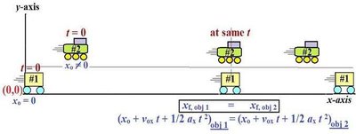
When analyzing the motion of multiple objects, their positions as functions of time can be set equal to find when and where they meet. This is especially useful in pursuit or collision problems.

• Example: Two trucks starting from different positions and/or velocities can be analyzed using their respective kinematic equations.

Piecewise Motion

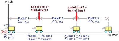
Sometimes, an object's motion is divided into segments with different accelerations or velocities. The final position and velocity from one segment become the initial conditions for the next.

• Example: A truck moves with different accelerations in three parts; the equations are applied sequentially for each part.

Vertical Motion Under Gravity

Objects moving vertically under the influence of gravity experience a constant acceleration downward, \( a_y = -9.8 \) m/s2. The same kinematic equations apply, with the acceleration directed along the y-axis.

• Example: A ball is thrown upward from a roof; its position and velocity at the top and when it hits the ground can be found using the equations of motion.

Additional info: The notes above expand on the provided images and formulas, adding context and definitions for clarity and completeness. All equations are presented in LaTeX format as required.