Motion Along a Straight Line

Position, Displacement, and Reference Frames

Understanding motion in one dimension begins with the concepts of position, displacement, and the reference frame. The position of an object is its location relative to a chosen origin, and displacement is the change in position over a time interval.

• Position (x): The location of an object along a straight line, measured from a reference point (origin).

• Displacement (Δx): The change in position, calculated as where is the final position and is the initial position.

• Reference Frame: The coordinate system used to define position and motion. All measurements of position, velocity, and acceleration are made relative to this frame.

• Direction: Displacement is a vector quantity and can be positive or negative depending on the chosen direction.

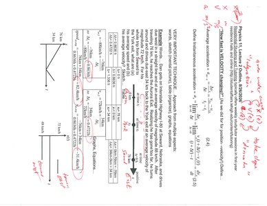
Average and Instantaneous Velocity

Velocity describes how fast and in what direction an object's position changes. The average velocity is the total displacement divided by the total time, while the instantaneous velocity is the velocity at a specific moment.

• Average Velocity ():

• Instantaneous Velocity ():

• Speed: The magnitude of velocity, always positive.

Velocity can be determined graphically as the slope of the position vs. time graph.

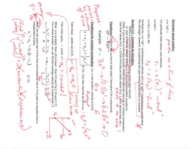
Acceleration: Average and Instantaneous

Acceleration measures how quickly velocity changes. Like velocity, it can be average or instantaneous.

• Average Acceleration ():

• Instantaneous Acceleration ():

• Acceleration is positive if velocity increases in the positive direction, negative if it decreases or increases in the negative direction.

On a velocity vs. time graph, acceleration is the slope.

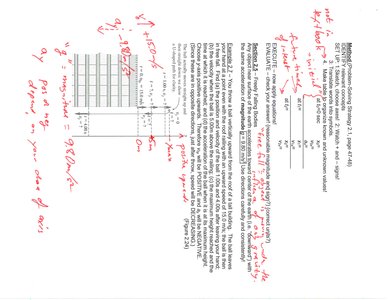
Kinematic Equations for Constant Acceleration

Equations and Their Use

When acceleration is constant, the following kinematic equations describe motion:

Where and are the initial position and velocity, is acceleration, and is time.

These equations are derived using calculus, integrating acceleration to get velocity and velocity to get position.

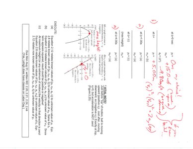
Example: Free Fall

Objects in free fall near Earth's surface experience constant acceleration due to gravity ( downward). The kinematic equations apply with (if upward is positive).

• Example: Dropping a ball from rest (), its position after time is .

Graphical Analysis of Motion

Interpreting Position, Velocity, and Acceleration Graphs

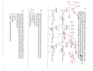
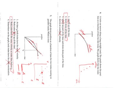
Graphs are powerful tools for visualizing and analyzing motion. The slope of a position-time graph gives velocity, and the slope of a velocity-time graph gives acceleration. The area under a velocity-time graph gives displacement.

• Constant velocity: straight line on position-time graph, horizontal line on velocity-time graph.

• Constant acceleration: parabolic position-time graph, straight line on velocity-time graph.

• Changing acceleration: curved velocity-time graph.

Problem Solving with Kinematics

Strategy and Example Problems

Solving kinematics problems involves identifying knowns and unknowns, choosing the appropriate equation, and carefully considering the direction of vectors. Drawing diagrams and labeling axes is essential for clarity.

• Step 1: Define the reference frame and assign positive direction.

• Step 2: List known quantities (initial position, velocity, acceleration, time).

• Step 3: Select the kinematic equation that relates the knowns to the unknown.

• Step 4: Solve algebraically, then substitute numbers.

• Step 5: Check units and physical reasonableness of the answer.

Example: A car accelerates from rest at for . Find its final velocity and displacement.

• Final velocity:

• Displacement:

Summary Table: Kinematic Quantities and Their Relationships

The following table summarizes the main kinematic quantities and their calculus relationships:

Additional info: The notes also include practice problems, graphical analysis, and strategies for interpreting and solving kinematics questions, which are foundational for all subsequent topics in Physics with Calculus.