Normal Distributions

Introduction to Normal Distributions

The normal distribution is one of the most important probability distributions in statistics. It describes data that cluster around a mean in a symmetric, bell-shaped curve. Many natural phenomena, such as heights or test scores, are approximately normally distributed.

• Relative frequency distributions can be visualized with histograms, which approximate the shape of the underlying distribution.

• As the measurement of a continuous variable becomes more precise (using smaller intervals), the histogram more closely resembles a smooth curve.

• The normal curve is a specific bell-shaped curve that is symmetric and defined by a precise mathematical formula.

Example: The distribution of adult women's heights is approximately normal, with most values clustering around the mean and fewer values as you move away from the center.

Continuous vs. Discrete Variables

A continuous variable can take any value within a range and can be measured to any desired level of precision. In contrast, a discrete variable can only take specific, separate values.

• Histograms of continuous variables become smoother as the interval width decreases.

• For example, grouping heights by tenths of an inch instead of whole inches produces a histogram that more closely approximates a curve.

Additional info: This property is not unique to normal distributions but applies to all continuous variables.

Parameters of the Normal Distribution

A normal distribution is completely determined by two parameters: the mean (\( \mu \)) and the standard deviation (\( \sigma \)).

• The mean (\( \mu \)) is the center of the distribution and also equals the mode and median due to symmetry.

• The standard deviation (\( \sigma \)) measures the spread or width of the curve.

• Smaller \( \sigma \): the curve is tall and narrow; larger \( \sigma \): the curve is short and wide.

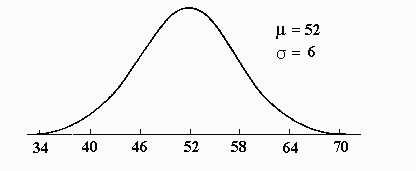
Example: The figure above shows a normal curve with \( \mu = 52 \) and \( \sigma = 6 \). The x-axis is marked at intervals of one standard deviation from the mean.

Comparing Normal Curves with Different Standard Deviations

Normal curves with the same mean but different standard deviations have the same center but different spreads.

• Curves with larger standard deviations are wider and flatter.

• Curves with smaller standard deviations are narrower and taller.

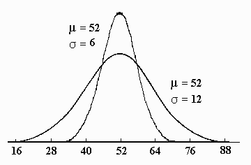
Example: The figure above compares two normal curves with \( \mu = 52 \), one with \( \sigma = 6 \) and the other with \( \sigma = 12 \).

Properties of the Normal Curve

The normal curve has several important properties:

• It is symmetric about the mean.

• The total area under the curve is 1 (representing 100% probability).

• Almost all the area (probability) lies within three standard deviations of the mean (from \( \mu - 3\sigma \) to \( \mu + 3\sigma \)).

• The curve approaches, but never touches, the horizontal axis as it extends infinitely in both directions.

The Standard Normal Distribution

Definition and Transformation

The standard normal distribution is a special case of the normal distribution with a mean of 0 and a standard deviation of 1. Any normal distribution can be converted to the standard normal distribution using z-scores.

• The z-score for a value \( x \) is calculated as:

• This transformation allows us to use standard normal tables to find probabilities for any normal distribution.

Properties of the Standard Normal Curve

• The total area under the curve is 1.

• The curve is symmetric about 0.

• Almost all the area lies between \( z = -3 \) and \( z = +3 \).

• Half the area (0.50) lies to the left of the mean (z = 0), and half to the right.

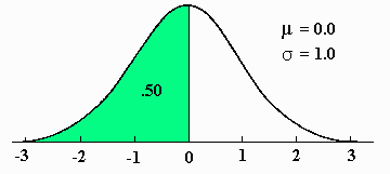
Example: The figure above shows the standard normal curve with the left half shaded, representing 50% of the area under the curve.

Summary Table: Properties of the Standard Normal Curve