Introduction to Business Statistics

Key Concepts and Terminology

Business statistics involves collecting, analyzing, and interpreting data to inform business decisions. Understanding the foundational terms and distinctions is essential for effective analysis.

• Data vs. Information: Data are raw facts; information is processed data used for decision-making.

• Primary vs. Secondary Data: Primary data is collected firsthand; secondary data is gathered by others.

• Qualitative vs. Quantitative: Qualitative data describes categories; quantitative data measures numerical values.

• Population vs. Sample: Population is the entire group of interest; sample is a subset used for analysis.

• Parameter vs. Statistic: Parameter describes a population; statistic describes a sample.

• Time Series vs. Cross-Sectional: Time series tracks one subject over time; cross-sectional compares multiple subjects at one time.

• Levels of Measurement (NOIR): Nominal (names), Ordinal (ordered), Interval (equal spacing, no true zero), Ratio (equal spacing, true zero).

Describing Data with Tables and Graphs

Frequency Distributions

Frequency distributions organize data into classes to reveal patterns and trends. Proper construction is crucial for accurate analysis.

• Number of Classes: Choose the smallest k such that .

• Class Width: (round up).

• Class Boundaries: Ensure boundaries are easy to read and non-overlapping.

• Frequency Types: Relative (frequency/total), Cumulative ("this value or less"), Ogive (line graph of cumulative frequency).

Class Rules: Equal widths, mutually exclusive, include every value, avoid empty/open-ended classes.

Describing Data Numerically

Measures of Central Tendency

Central tendency measures summarize data with a single value representing the center of the distribution.

• Mean: Default for numeric data; sensitive to outliers. Weighted mean: .

• Median: Use with skewed data or outliers. Find by sorting and locating the middle value.

• Mode: Most frequent value; only option for categorical data.

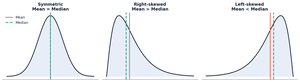
Measures of Spread and z-Scores

Spread measures describe variability in data. z-scores standardize values for comparison.

• Sample vs. Population Variance: Sample divides by , population by .

• Coefficient of Variation: ; lower CV indicates more consistency.

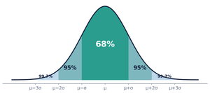
• z-Score: ; values beyond ±3 are outliers.

Probability

Rules and Tools

Probability quantifies uncertainty. Different rules apply based on event relationships.

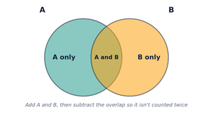
• OR Rule: ; drop last term if mutually exclusive.

• AND Rule: ; if independent, .

• GIVEN Rule: .

• Complement Rule: ; "at least one" is .

Contingency Tables

Contingency tables display joint, marginal, and conditional probabilities for categorical data.

• Marginal: Row/column total ÷ grand total.

• Joint: One cell ÷ grand total.

• Conditional: Restrict to given row/column.

Discrete and Continuous Distributions

Choosing the Right Distribution

Identifying the correct distribution is essential for accurate probability calculations. Distributions are classified as discrete (counted) or continuous (measured).

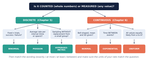
• Binomial: Fixed trials, two outcomes, constant probability.

• Poisson: Counts events per interval; average rate.

• Hypergeometric: Sampling without replacement from a small group.

• Normal: Bell-shaped, mean and SD given.

• Exponential: Time between events.

• Uniform: All values equally likely between a and b.

Binomial, Poisson, and Hypergeometric Distributions

Binomial Distribution

Used for a fixed number of trials with two outcomes (success/failure) and constant probability.

• Probability:

• Mean:

• Standard Deviation:

Poisson Distribution

Models the number of events in a fixed interval at an average rate .

• Probability:

• Mean and SD: ,

Hypergeometric Distribution

Used for sampling without replacement from a finite population.

• Probability:

• Mean:

Normal Distribution & Continuous Random Variables

Normal Distribution

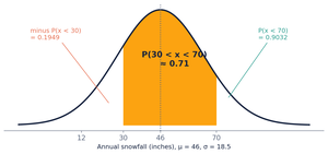
The normal distribution is bell-shaped and characterized by its mean () and standard deviation (). It is used to model many natural phenomena.

• z-Score:

• Empirical Rule: 68% within ±1 SD, 95% within ±2 SD, 99.7% within ±3 SD.

• Finding Probabilities: Convert to z, use table for area to the left, adjust for wording.

Normal Approximation to the Binomial

When and , the binomial can be approximated by the normal distribution.

• Mean:

• SD:

• Continuity Correction: Add/subtract 0.5 to whole-number counts.

Exponential and Uniform Distributions

Exponential Distribution

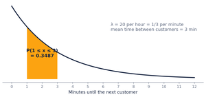
Models the time between events in a Poisson process. It is right-skewed and never negative.

• Probability: , ,

• Mean and SD:

Uniform Distribution

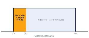
All values between a and b are equally likely. Used for modeling situations with constant probability across an interval.

• Probability:

• Mean:

• SD:

Worked Examples and Approximations

Binomial vs. Poisson Approximation

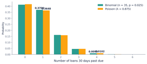
Poisson can approximate binomial when and , with . Approximations are close but not identical.

Normal Distribution: Area Between Two Values

To find the probability between two values, subtract the area to the left of the lower value from the area to the left of the upper value.

Exponential Distribution: Time Between Events

For time between events, use the exponential formula and ensure units match the rate parameter.

Uniform Distribution: Probability Within an Interval

For uniform distributions, calculate the probability as the fraction of the interval width.

Summary Table: Distribution Properties

Exam Tips and Habits

Effective Strategies

• Bank free points: Write definitions first.

• Name the tool: Identify the distribution before calculating.

• Highlight direction words: exactly, at most, at least, between.

• Convert units: Always match units before calculation.

• Use complements: "At least one" is often .

• Don't round early: Keep four decimals until the final answer.

• Sketch and shade: Visualize normal and exponential problems.

• Reality-check: Probabilities must be between 0 and 1.

• Counting events: Use Poisson; time until next event: exponential.

• Check cumulative settings: TRUE for cumulative, FALSE for exact.