Descriptive Statistics

Introduction

Descriptive statistics provide essential tools for summarizing and describing the main features of a data set. Both graphical and numerical summaries are used to explore data, offering insights into central tendency, dispersion, and relationships between variables.

Measures of Central Tendency

Arithmetic Mean

The arithmetic mean (or simply mean) is the average of all values in a data set and is the most commonly used measure of central tendency.

• Formula for a sample mean:

• Sensitive to outliers: Extreme values can significantly affect the mean.

• Example: For the data set 0, 1, 2, 3, 4, 5, 6, 7, 8, 9, 10, the mean is 5.

Median

The median is the middle value in an ordered data set, with 50% of values above and 50% below. It is not affected by extreme values.

• Finding the median:

  • If n is odd, the median is the middle value.

  • If n is even, the median is the average of the two middle values.

• Median position:

Mode

The mode is the value that appears most frequently in a data set. It is useful for discrete numerical or categorical data and is not affected by outliers.

• There may be no mode, one mode, or several modes.

Geometric Mean

The geometric mean is used for sets of positive numbers and is especially useful for growth rates and financial returns.

• Formula:

Trimmed Mean

The trimmed mean is calculated by removing a specified percentage of the highest and lowest values before computing the mean. This reduces the impact of outliers.

• Example: A 10% trimmed mean removes the lowest and highest 10% of values before averaging.

Percentiles and Quartiles

Percentiles

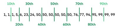
Percentiles indicate the value below which a given percentage of observations fall. For example, the 90th percentile is the value below which 90% of the data lie.

Quartiles

Quartiles divide ordered data into four equal parts:

• Q1: 25% of data below

• Q2: 50% (the median)

• Q3: 75% of data below

Formulas for quartile positions:

• Q1:

• Q2:

• Q3:

Box-and-Whisker Plot

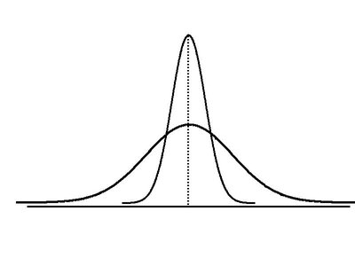
A box-and-whisker plot visually displays the five-number summary: minimum, Q1, median, Q3, and maximum.

Measures of Variation

Range

The range is the difference between the largest and smallest values in a data set:

• Formula: Range =

• Simple but sensitive to outliers.

Interquartile Range (IQR)

The interquartile range (IQR) measures the spread of the middle 50% of data and is less affected by outliers:

• Formula:

Variance and Standard Deviation

Variance and standard deviation measure the average squared deviation and the average deviation from the mean, respectively.

• Population variance:

• Sample variance:

• Population standard deviation:

• Sample standard deviation:

Coefficient of Variation (CV)

The coefficient of variation expresses the standard deviation as a percentage of the mean, allowing comparison between data sets with different units or means:

• Formula:

Shape of Distribution

Skewness

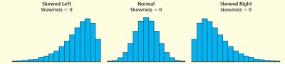
Skewness measures the asymmetry of a distribution:

• Skewness < 0: Left-skewed

• Skewness = 0: Symmetric

• Skewness > 0: Right-skewed

Kurtosis

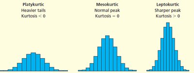
Kurtosis measures the "peakedness" of a distribution:

• Kurtosis < 0: Platykurtic (flatter)

• Kurtosis = 0: Mesokurtic (normal)

• Kurtosis > 0: Leptokurtic (sharper peak)

Standardized Data (Z-Scores)

Z-Score

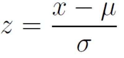
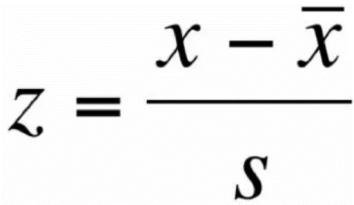
A z-score indicates how many standard deviations a value is from the mean. It is used to compare values from different distributions or to identify outliers.

• Population z-score:

• Sample z-score:

Chebyshev's Theorem and Empirical Rule

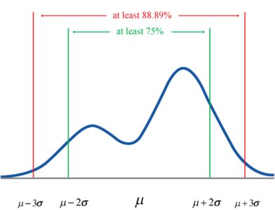
These rules help estimate the proportion of data within a certain number of standard deviations from the mean.

• Chebyshev's Theorem: For any distribution, at least of values lie within standard deviations of the mean (for ).

• Empirical Rule (for bell-shaped distributions):

  • About 68% within

  • About 95% within

  • About 99.7% within

Outliers

Outliers are observations that lie far from the rest of the data, often defined as values more than 3 standard deviations from the mean or outside the outer fences in a boxplot.

Grouped Data

Weighted Mean and Approximations

For grouped data, the mean and variance can be approximated using class midpoints and frequencies.

• Weighted mean:

• Variance for grouped data:

Linear Relationship: Covariance and Correlation

Covariance

Covariance measures the direction of the linear relationship between two variables.

• Sample covariance:

• cov(X,Y) > 0: X and Y move in the same direction

• cov(X,Y) < 0: X and Y move in opposite directions

• cov(X,Y) = 0: X and Y are independent

Correlation Coefficient

The correlation coefficient (r) measures the strength and direction of the linear relationship between two variables. It is unit-free and ranges from -1 to 1.

• Formula:

• r = 1: Perfect positive linear relationship

• r = -1: Perfect negative linear relationship

• r = 0: No linear relationship

Scatter Plots

Scatter plots visually display the relationship between two quantitative variables, helping to identify the direction and strength of their association.

Using Excel for Descriptive Statistics

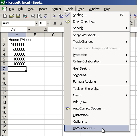
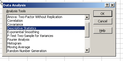
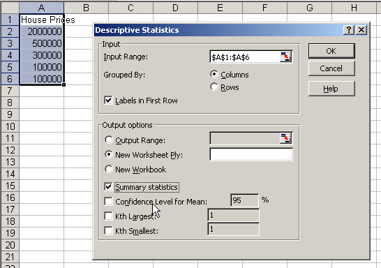
Microsoft Excel provides tools for calculating descriptive statistics, including mean, median, mode, standard deviation, variance, skewness, and kurtosis.

Summary Table: Key Measures