Discrete Probability Distributions

Random Variables

A random variable is a function that assigns a numerical value to each outcome in the sample space of a random experiment. Random variables are fundamental in statistics for quantifying outcomes and analyzing probability distributions.

• Discrete random variable: Takes countable values (e.g., number of heads in coin tosses).

• Continuous random variable: Takes values from a continuum (e.g., height, waiting time).

• Sample space: The set of all possible outcomes of an experiment.

Example: Tossing a fair coin three times, the random variable X could represent the number of heads observed.

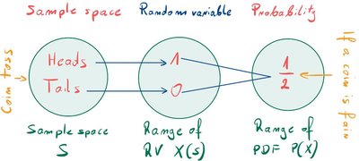
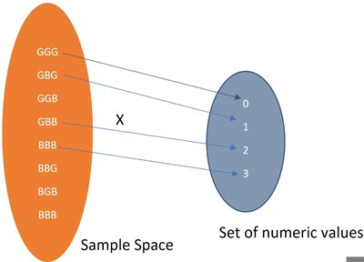
Additional info: Discrete random variables are often used in business statistics to model counts, such as the number of defective products or customer arrivals.

Probability Distributions of a Random Variable

A probability distribution describes the likelihood of each possible value of a random variable. For discrete random variables, this is often represented as a probability mass function (PMF) or a probability table.

• Probability Mass Function (PMF): Assigns probabilities to each possible value of a discrete random variable.

• Probability tables: List all possible values and their associated probabilities.

• Graphical representation: Bar charts or histograms are commonly used to visualize discrete distributions.

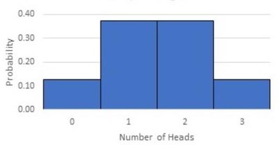
Example: Tossing a fair coin three times, the probability distribution for the number of heads is shown below.

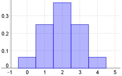
Example: Tossing a fair coin four times, the probability distribution for the number of heads is shown below.

Discrete Probability Density Function and Cumulative Distribution Function

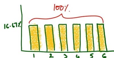
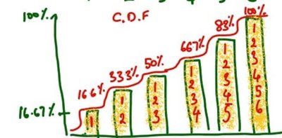
The Probability Density Function (PDF) for discrete random variables is the PMF, which gives the probability for each value. The Cumulative Distribution Function (CDF) gives the probability that the random variable is less than or equal to a certain value.

• PDF: for each value x.

• CDF: , the sum of probabilities up to x.

Expected Value and Variance

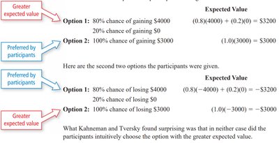
The expected value (mean) of a random variable is a measure of its central tendency, while the variance measures the spread of its values.

• Expected value formula:

• Variance formula:

• Standard deviation:

Example: Calculating expected value for a lottery ticket or insurance policy helps businesses assess risk and profitability.

Common Discrete Probability Distributions

Several discrete probability distributions are commonly used in business statistics:

• Uniform Distribution: All outcomes are equally likely.

• Binomial Distribution: Models the number of successes in n independent trials with probability p.

• Hypergeometric Distribution: Models the number of successes in n dependent trials (without replacement).

• Geometric Distribution: Models the number of trials until the first success.

• Poisson Distribution: Models the number of events in a fixed interval of time or space.

Uniform Distribution

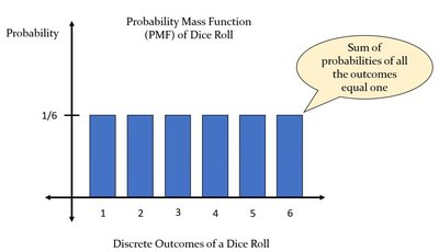
The uniform distribution assigns equal probability to each outcome. For example, rolling a fair die, each number from 1 to 6 has probability 1/6.

• PMF: for n possible outcomes.

Example: In a lottery, each number is equally likely to be drawn.

Binomial Distribution

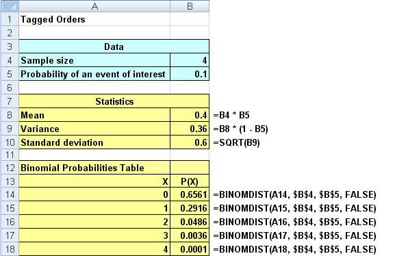
The binomial distribution models the number of successes in n independent trials, each with probability p of success.

• Parameters: n = number of trials, p = probability of success.

• PMF:

• Mean:

• Variance:

Example: Probability of 2 uninsured patients in a sample of 4, given 20% lack insurance.

Hypergeometric Distribution

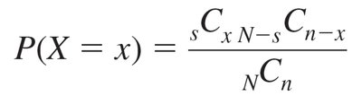
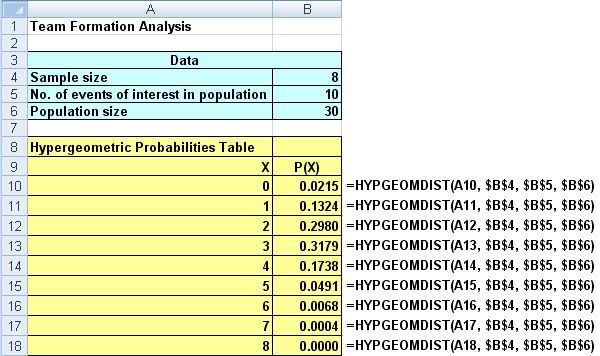
The hypergeometric distribution models the number of successes in n draws from a finite population without replacement.

• Parameters: N = population size, s = number of successes in population, n = sample size, x = number of successes in sample.

• PMF:

Poisson Distribution

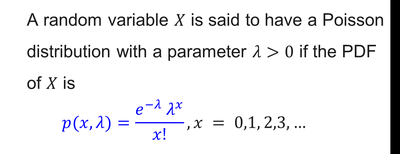
The Poisson distribution models the number of events occurring in a fixed interval of time or space, given the average rate λ.

• Parameter: = average number of events per interval.

• PMF:

• Mean and variance: Both equal to .

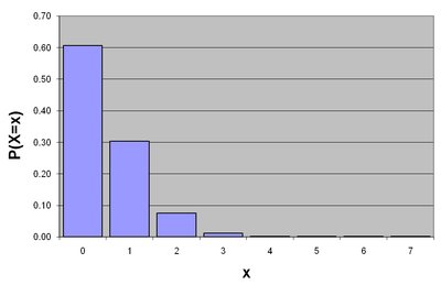
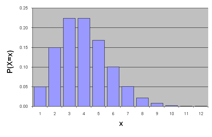
Example: Probability of 3 houses sold in a day when average is 2.

Additional info: Poisson distribution is used for modeling rare events, such as defects in manufacturing or customer arrivals.

Comparisons and Approximations

Sometimes, one distribution can approximate another under certain conditions:

• Poisson approximation to binomial: When n is large and p is small, binomial can be approximated by Poisson with .

• Binomial approximation to hypergeometric: When sample size n is small relative to population N (), hypergeometric can be approximated by binomial.

Example: Calculating the probability of no mishandled bags among 500 students, given a small probability per bag.

Additional info: These approximations simplify calculations in business applications, such as quality control and auditing.

Summary Table: Common Discrete Distributions

End of Topic