Counting Rules

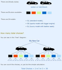
Basic Principle of Counting

Counting rules are essential for determining the number of possible outcomes in various business and statistical scenarios. The fundamental principle states that if an experiment consists of r sequential steps, with n1 possible outcomes for the first step, n2 for the second, and so on, then the total number of possible outcomes is the product:

• Example: Choosing a car with 2 body styles, 5 colors, and 3 models yields possible choices.

Permutations

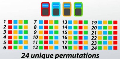
A permutation is an ordered arrangement of objects. The number of ways to arrange n distinct objects is:

• r-Permutation: The number of ways to arrange r objects out of n is:

• Example: Arranging 4 colored blocks in all possible orders yields 24 unique permutations.

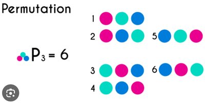
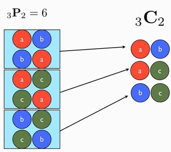
• Example: Arranging 3 colored balls in all possible orders yields 6 permutations.

Combinations

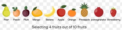
A combination is a selection of objects where order does not matter. The number of ways to choose r objects from n is:

• Example: Selecting 4 fruits out of 10 possible fruits.

• Comparison: Permutations consider order, combinations do not.

Special Counting Principles

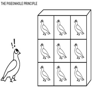
• Pigeonhole Principle: If more objects are placed into fewer boxes, at least one box contains more than one object. Useful for minimum guarantees in probability.

Binomial and Multinomial Theorems

The Binomial Theorem expands expressions of the form :

The Multinomial Theorem generalizes this to more than two terms:

• Application: Used in probability for binomial and multinomial distributions.

Probability Concepts

Random Experiments and Sample Spaces

A random experiment is a process with uncertain outcomes. The sample space (S) is the set of all possible outcomes.

• Discrete sample space: Countable outcomes (e.g., rolling a die).

• Continuous sample space: Uncountable outcomes (e.g., waiting time).

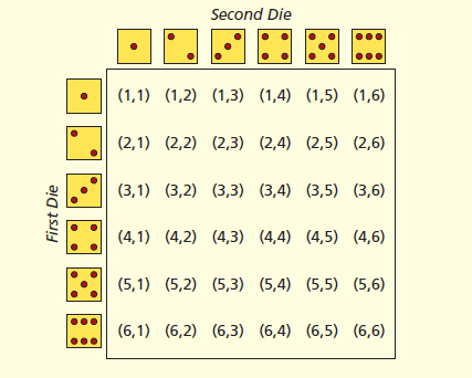
• Example: Rolling two dice yields 36 possible outcomes.

• Example: Flipping a coin twice yields 4 possible outcomes: HH, HT, TH, TT.

Events

• Simple event: Contains a single outcome (e.g., rolling a 3).

• Compound event: Contains multiple outcomes (e.g., rolling an even number).

Probability of an Event

The probability of an event is a number between 0 and 1 representing its likelihood. It can also be expressed as a percentage.

The probability of event A is denoted as .

Approaches to Probability

• Subjective Probability: Based on personal judgment or experience.

• Classical Probability: Based on equally likely outcomes (e.g., games of chance).

• Empirical Probability: Based on observed data or relative frequency.

Rules of Probability

Complement Rule

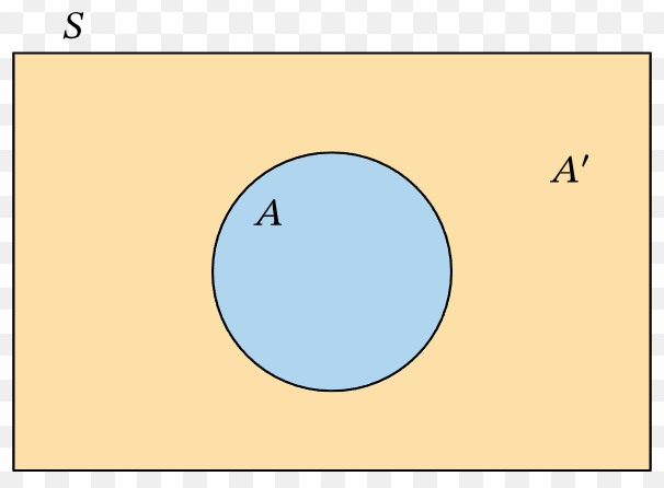
The complement of event A, denoted or , includes all outcomes not in A. The probability is:

Intersection and Union of Events

• Intersection (A ∩ B): Outcomes common to both A and B. Probability is (joint probability).

• Union (A ∪ B): Outcomes in A, B, or both. Probability is .

General Law of Addition

The probability of the union of two events is:

• If A and B are mutually exclusive: , so .

Mutually Exclusive and Collectively Exhaustive Events

• Mutually exclusive: Events cannot occur together ().

• Collectively exhaustive: At least one event must occur; their union covers the entire sample space.

Conditional Probability and Independence

Conditional Probability

The probability of event A given that event B has occurred is:

• Multiplication Rule:

Independent and Dependent Events

• Independent: The occurrence of one event does not affect the probability of the other.

• Dependent: The occurrence of one event affects the probability of the other.

Odds of an Event

The odds in favor of event A is the ratio of the probability that A occurs to the probability that A does not occur:

The odds against event A is the reciprocal:

Contingency Tables and Decision Trees

Contingency Tables

Contingency tables display the frequency or probability of combinations of two or more categorical variables. They are useful for calculating marginal, joint, and conditional probabilities.

Decision Trees

Decision trees visually represent sequences of events and their probabilities, aiding in the calculation of joint and conditional probabilities in multi-stage experiments.

Bayes’ Theorem

Bayes’ Theorem allows us to update probabilities based on new information. It is derived from the definition of conditional probability and the law of total probability:

• Application: Used in business for diagnostic testing, quality control, and decision-making under uncertainty.

Summary Table: Key Probability Rules

Additional info: These foundational concepts are critical for understanding probability models, risk assessment, and statistical inference in business contexts.