Macroeconomic Theory: Exam 1 Review

Overview of Exam 1

This review covers the foundational concepts in macroeconomics as presented in Chapters 1–6. The focus is on the short run, including the goods and financial markets, the IS-LM model, and the role of expectations and risk in macroeconomic analysis. Students should be prepared for multiple question types, including essays, multiple choice, true/false, graphical analysis, and mathematical problems.

Chapter 1: A Tour of the World

Macroeconomics Since Keynes

• Keynes’s General Theory revolutionized macroeconomics by focusing on aggregate demand and the role of government policy in stabilizing the economy.

• Disagreement Among Economists: Differences arise from varying theoretical perspectives, empirical evidence, and policy priorities.

• Key Macro Variables: Output (GDP), unemployment, inflation, and public debt are central to macroeconomic analysis.

• Contemporary Issues: The COVID-19 pandemic, rising public debt, China’s economic growth, inequality, and global warming are major macroeconomic challenges.

Chapter 2: A Tour of the Book

Measuring Economic Activity

• GDP (Gross Domestic Product): The value of all final goods and services produced within a country during a given period.

• Methods of Measuring GDP:

  • Aggregate production (sum of value added)

  • Aggregate income

  • Aggregate expenditures (demand)

• Nominal vs. Real GDP: Nominal GDP is measured at current prices; real GDP is adjusted for inflation.

• Inflation Adjustment: Necessary for comparing economic output over time, but can be challenging due to changing price levels and quality of goods.

Labor Market Indicators

• Unemployment and Employment: The labor force includes all employed and unemployed individuals actively seeking work.

• Participation Rate: The proportion of the working-age population in the labor force.

• Unemployment Rate: The percentage of the labor force that is unemployed.

• Discouraged Workers: Individuals not actively seeking work due to poor job prospects.

Inflation and Price Indices

• Inflation: The rate at which the general price level of goods and services rises.

• Deflation: A decrease in the general price level.

• Price Stability: Low and stable inflation is a key macroeconomic goal.

• GDP Deflator: Measures the price level of all domestically produced goods and services.

• Consumer Price Index (CPI): Measures the average change in prices paid by consumers for a basket of goods and services.

Relationships Among Key Variables

• Okun’s Law: Empirical relationship between GDP growth and changes in the unemployment rate. When GDP grows faster than trend, unemployment falls.

• The Phillips Curve: Describes the inverse relationship between unemployment and inflation in the short run. The equilibrium unemployment rate is where inflation remains stable.

Chapter 3: The Goods Market

Aggregate Demand and Output Determination

• Short Run: Output is determined by aggregate demand; one person’s spending is another’s income.

• Goods Market Equilibrium: Occurs when planned spending equals output produced.

• Investment (I) and Saving (S): In equilibrium, investment equals saving ().

• Closed Economy: No international trade; all spending is domestic.

The Consumption Function

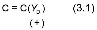
The consumption function models the relationship between disposable income and consumption:

• Endogenous Variable: Consumption depends on income.

• Exogenous Variables: Investment, government spending, and taxes are taken as given in the basic model.

Aggregate Demand and the Multiplier

• Aggregate Demand: The total demand for goods and services in the economy.

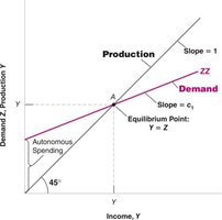
• Equilibrium Output: Determined where production equals demand.

• The Multiplier: Measures how much equilibrium output changes in response to a change in autonomous spending. The multiplier is larger when the marginal propensity to consume () is closer to 1.

Graphical Representation: The Keynesian Cross

The Keynesian cross diagram shows equilibrium where the aggregate demand (ZZ) curve intersects the 45-degree line (where output equals demand). An increase in autonomous spending leads to a multiplied increase in equilibrium output.

Saving Behavior and the Paradox of Thrift

• Precautionary Saving: In times of uncertainty, households may increase saving, reducing aggregate demand.

• Paradox of Saving: If everyone tries to save more, aggregate demand falls, leading to lower income and possibly lower total saving.

• Balanced-Budget Multiplier: Even with a balanced government budget, changes in spending and taxes can affect output.

Chapter 4: Financial Markets I

The Role of Finance and Central Banking

• Central Bank (CB): Influences interest rates and financial conditions through monetary policy.

• Types of Money: Banknotes (issued by government) and bank deposits (created by private banks).

• Motives for Holding Money: Transactions and as a store of wealth (alternative to bonds).

• Determinants of Money Demand: Level of transactions (GDP) and the interest rate on bonds (opportunity cost of holding money).

Money Market Equilibrium

• Money Demand Curve: Lower interest rates increase the demand for money; higher income shifts the demand curve right.

• Central Bank Policy: The CB typically sets a policy interest rate (e.g., the Fed Funds rate) and accommodates the demand for reserves at that rate.

• Liquidity Trap: When the policy rate hits zero, holding money has no opportunity cost, limiting the effectiveness of monetary policy (horizontal money demand curve).

• Quantitative Easing (QE): When at the zero lower bound, the CB may purchase assets to lower long-term interest rates.

Chapter 5: The IS-LM Model

Investment, Interest Rates, and the IS Curve

• Investment Function: Investment depends on output (Y) and the interest rate (i).

• IS Curve: Shows combinations of output and interest rates where the goods market is in equilibrium. It is downward sloping because higher interest rates reduce investment and output.

• Shifts in the IS Curve: Changes in fiscal policy (e.g., taxes, government spending) shift the IS curve.

Financial Markets and the LM Relation

• LM Curve: Shows combinations of output and interest rates where the money market is in equilibrium. In modern analysis, the LM curve is often depicted as horizontal at the policy interest rate set by the central bank.

• Equilibrium: The intersection of the IS and LM curves determines the equilibrium output and interest rate.

Policy Analysis in the IS-LM Model

• Fiscal Policy: Changes in government spending (G) and taxes (T) shift the IS curve.

• Monetary Policy: Changes in the money supply or policy interest rate shift the LM curve.

• Policy Mix: The combination of fiscal and monetary policies used to achieve macroeconomic objectives.

Chapter 6: Financial Markets II

Extending the IS-LM Model

• Price Level and Expectations: The price level can change over time, and economic agents form expectations about future inflation.

• Nominal vs. Real Interest Rates: The real interest rate adjusts the nominal rate for expected inflation.

• Risk Premium: The extra return required by investors to hold risky assets, reflecting default risk and risk aversion.

• Financial Intermediation: Banks and other intermediaries channel funds from savers to borrowers, create money, and manage risks.

The Real Interest Rate

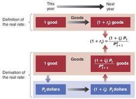
The real interest rate reflects the true cost of borrowing after accounting for inflation. It is crucial for consumption and investment decisions.

• Formula:

  • One-year real interest rate:

  • Approximation:

• Because expected inflation is usually positive, the real interest rate is typically lower than the nominal rate.

Risk and Risk Premia

• Risk Premium (x): Determined by the probability of default and the degree of risk aversion among investors.

• Arbitrage Equilibrium: The expected return on risky bonds must exceed that on riskless bonds by the risk premium.

• Formula:

Banks and Financial Intermediation

• Banks: Special financial intermediaries that create money by making loans and taking deposits.

• Limits to Lending: Banks face default risk, leverage constraints, and liquidity risks.

• Lender of Last Resort: The central bank provides system liquidity to prevent bank runs and systemic crises.

Financial Shocks and Policy Response

• Financial Shocks: Increase risk premia and shift the IS curve left, reducing output.

• Monetary Policy Response: Lowering the policy rate can offset higher risk premia, but the zero lower bound may limit effectiveness.

• Great Financial Crisis (GFC): The crisis shifted the IS curve left; policy responses shifted IS and LM curves but were insufficient to prevent a major recession.