뒤로
Chapter 13: The Costs of Production – Microeconomics Study Notes
스터디 가이드 - 스마트 노트
 자료에 맞춘 맞춤형 노트, 핵심 정의, 예시, 맥락을 확장해 제공합니다.
The Costs of Production
Introduction
This chapter explores how firms measure and analyze the costs associated with producing goods and services. Understanding these costs is essential for making rational business decisions and maximizing profit.
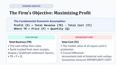
The Firm's Objective: Maximizing Profit
Profit and Its Calculation
Firms aim to maximize profit, which is the difference between total revenue and total cost.
Profit (π) = Total Revenue (TR) – Total Cost (TC)
Total Revenue (TR): The cash inflow from sales, calculated as TR = Price (P) × Quantity (Q).
Total Cost (TC): The market value of all inputs used in production, including both explicit and implicit costs.
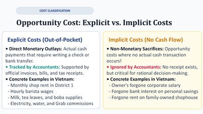
Opportunity Cost: Explicit vs. Implicit Costs
Types of Costs
Explicit Costs: Out-of-pocket payments for resources (e.g., wages, rent, materials). These are tracked by accountants.
Implicit Costs: Non-monetary opportunity costs, such as the owner's time or foregone interest. These are not recorded by accountants but are crucial for economic decision-making.
Example: In Vietnam, explicit costs might include shop rent and supplies, while implicit costs could be the owner's forgone salary or rent on a family-owned property.
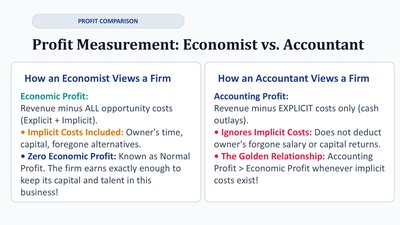
Profit Measurement: Economist vs. Accountant
Different Perspectives
Economic Profit: Revenue minus all opportunity costs (explicit + implicit). Includes the value of the owner's time and capital.
Accounting Profit: Revenue minus only explicit costs (cash outlays). Ignores implicit costs.
Relationship: Accounting profit is always greater than or equal to economic profit.
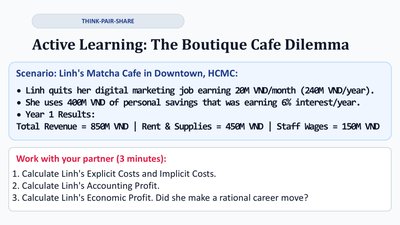
Active Learning: The Boutique Cafe Dilemma
Case Study Example
Scenario: Linh quits her job to open a cafe, using her savings. Students are asked to calculate explicit and implicit costs, accounting profit, and economic profit based on provided data.
Explicit Costs: Rent, supplies, staff wages
Implicit Costs: Foregone salary, interest on savings
Accounting Profit: TR – Explicit Costs
Economic Profit: TR – (Explicit + Implicit Costs)
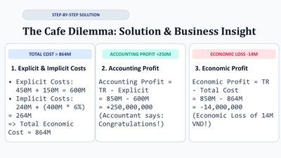
The Cafe Dilemma: Solution & Business Insight
Step-by-Step Calculation
Total Economic Cost: Sum of explicit and implicit costs
Accounting Profit:
Economic Profit:
Insight: A positive accounting profit does not guarantee a positive economic profit.
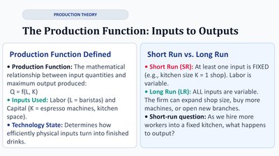
The Production Function: Inputs to Outputs
Production Function Defined
Production Function: Mathematical relationship between input quantities and maximum output:
Inputs: Labor (L), Capital (K)
Short Run (SR): At least one input is fixed
Long Run (LR): All inputs are variable
Marginal Product of Labor (MP_L)
Definition and Calculation
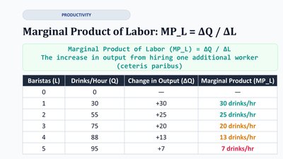
Marginal Product of Labor (MP_L): The increase in output from hiring one additional worker, holding other inputs constant.
Formula:
Baristas (L) | Drinks/Hour (Q) | Change in Output (ΔQ) | Marginal Product (MP_L) |
|---|---|---|---|
0 | 0 | +30 | 30 drinks/hr |
1 | 30 | +25 | 25 drinks/hr |
2 | 55 | +20 | 20 drinks/hr |
3 | 75 | +13 | 13 drinks/hr |
4 | 88 | +7 | 7 drinks/hr |
5 | 95 |
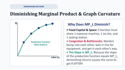
Diminishing Marginal Product & Graph Curvature
Why Does MP_L Diminish?
Fixed Capital & Space: Limited equipment and space cause workers to become less productive as more are hired.
Congestion & Bottlenecks: Workers interfere with each other, reducing the marginal product.
Graph: The production function curve gets flatter as more labor is added.
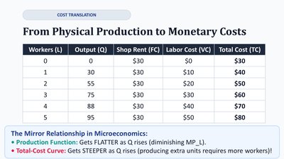
From Physical Production to Monetary Costs
Translating Output to Costs
Workers (L) | Output (Q) | Shop Rent (FC) | Labor Cost (VC) | Total Cost (TC) |
|---|---|---|---|---|
0 | 0 | $30 | $0 | $30 |
1 | 30 | $30 | $10 | $40 |
2 | 55 | $30 | $20 | $50 |
3 | 75 | $30 | $30 | $60 |
4 | 88 | $30 | $40 | $70 |
5 | 95 | $30 | $50 | $80 |
Mirror Relationship: As output rises, the production function flattens (diminishing MP_L), while the total-cost curve gets steeper (increasing marginal cost).
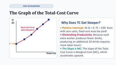
The Graph of the Total-Cost Curve
Cost Curve Characteristics
Positive Intercept: Fixed costs must be paid even at zero output.
Diminishing Productivity: More labor is needed for each additional unit of output, making the total-cost curve steeper.
Slope: The slope of the total-cost curve is the marginal cost (MC).
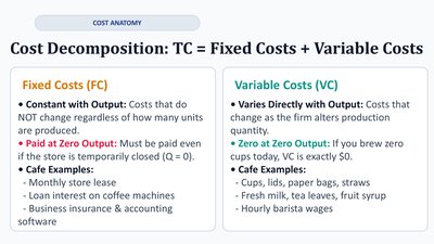
Cost Decomposition: TC = Fixed Costs + Variable Costs
Types of Costs
Fixed Costs (FC): Do not change with output (e.g., rent, insurance). Must be paid even if output is zero.
Variable Costs (VC): Change with output (e.g., materials, hourly wages). Zero if output is zero.
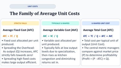
The Family of Average Unit Costs
Types of Average Costs
Average Fixed Cost (AFC): – Falls as output increases.
Average Variable Cost (AVC): – Typically U-shaped due to specialization and diminishing returns.
Average Total Cost (ATC): – U-shaped; used to compare with market price for profitability.
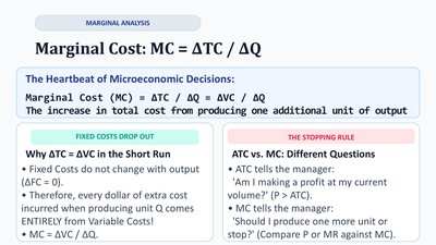
Marginal Cost: MC = ΔTC / ΔQ
Marginal Analysis
Marginal Cost (MC): The increase in total cost from producing one additional unit of output.
Formula:
Fixed Costs Drop Out: In the short run, only variable costs change with output.
ATC vs. MC: ATC tells if the firm is profitable at current output; MC helps decide whether to produce more or less.
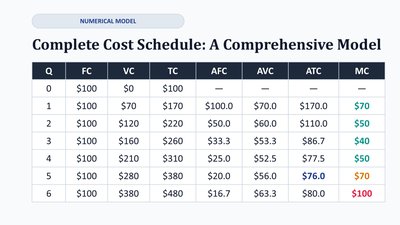
Complete Cost Schedule: A Comprehensive Model
Numerical Example
Q | FC | VC | TC | AFC | AVC | ATC | MC |
|---|---|---|---|---|---|---|---|
0 | $100 | $0 | $100 | – | – | – | – |
1 | $100 | $70 | $170 | $100.0 | $70.0 | $170.0 | $70 |
2 | $100 | $120 | $220 | $50.0 | $60.0 | $110.0 | $50 |
3 | $100 | $160 | $260 | $33.3 | $53.3 | $86.7 | $40 |
4 | $100 | $200 | $300 | $25.0 | $50.0 | $75.0 | $40 |
5 | $100 | $280 | $380 | $20.0 | $56.0 | $76.0 | $70 |
6 | $100 | $380 | $480 | $16.7 | $63.3 | $80.0 | $100 |
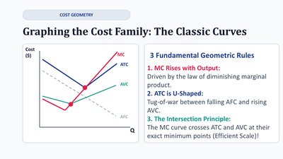
Graphing the Cost Family: The Classic Curves
Geometric Rules
MC Rises with Output: Due to diminishing marginal product.
ATC is U-Shaped: Result of falling AFC and rising AVC.
Intersection Principle: MC crosses ATC and AVC at their minimum points (efficient scale).
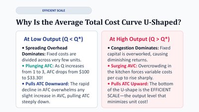
Why Is the Average Total Cost Curve U-Shaped?
Explanation of the U-Shape
At Low Output: Spreading overhead dominates, causing AFC to fall rapidly and pulling ATC down.
At High Output: Congestion dominates, causing AVC to rise and pulling ATC up.
Efficient Scale: The output level that minimizes unit cost (bottom of the U-shape).
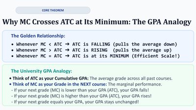
Why MC Crosses ATC at Its Minimum: The GPA Analogy
The Golden Relationship
Whenever MC < ATC, ATC is falling.
Whenever MC > ATC, ATC is rising.
Whenever MC = ATC, ATC is at its minimum (efficient scale).
Analogy: Think of ATC as your cumulative GPA and MC as your next course grade. If your next grade is below your GPA, your GPA falls; if above, it rises; if equal, it stays unchanged.