뒤로
Firms in Competitive Markets: Microeconomics Study Notes
스터디 가이드 - 스마트 노트
 자료에 맞춘 맞춤형 노트, 핵심 정의, 예시, 맥락을 확장해 제공합니다.
Firms in Competitive Markets
Introduction
This chapter explores the behavior of firms in perfectly competitive markets, focusing on how they maximize profit, make shutdown and exit decisions, and achieve long-run equilibrium. Key concepts include price taking, marginal analysis, and the relationship between costs and supply.
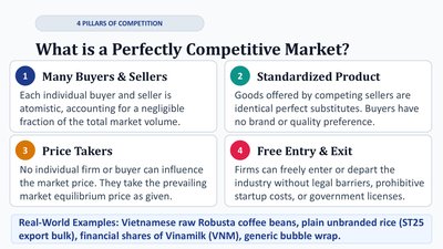
What is a Perfectly Competitive Market?
Four Pillars of Competition
Many Buyers & Sellers: Each participant is so small relative to the market that no single buyer or seller can influence the market price.
Standardized Product: All firms offer identical goods, making products perfect substitutes with no brand or quality differentiation.
Price Takers: Firms and buyers accept the market equilibrium price; no individual can set prices.
Free Entry & Exit: Firms can enter or leave the market without significant barriers, ensuring long-term market flexibility.
Examples: Vietnamese raw Robusta coffee beans, plain unbranded rice, financial shares of Vinamilk, generic bubble wrap.
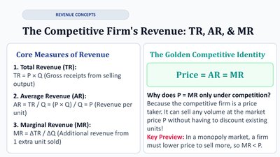
The Competitive Firm's Revenue: TR, AR, & MR
Core Measures of Revenue
Total Revenue (TR): (Gross receipts from selling output)
Average Revenue (AR): (Revenue per unit)
Marginal Revenue (MR): (Additional revenue from selling one more unit)
The Golden Competitive Identity: Price = AR = MR
This identity holds because competitive firms are price takers and can sell any quantity at the market price without affecting it.
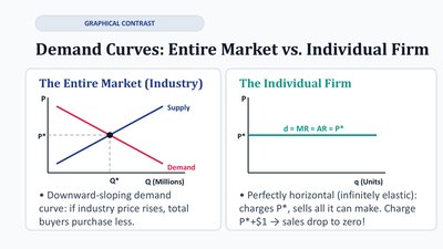
Demand Curves: Entire Market vs. Individual Firm
Graphical Contrast
Entire Market (Industry): The market demand curve is downward sloping; higher prices reduce total quantity demanded.
Individual Firm: The firm's demand curve is perfectly horizontal (infinitely elastic) at the market price. Any attempt to charge more results in zero sales.
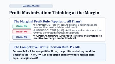
Profit Maximization: Thinking at the Margin
Marginal Profit Rule
If MR > MC: Expand output (increase Q) to add profit.
If MR < MC: Reduce output (decrease Q) to avoid losses.
If MR = MC: Profit is maximized; no incentive to change output.
Competitive Firm's Decision Rule: Set output where .
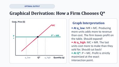
Graphical Derivation: How a Firm Chooses Q*
Optimal Output
At low output (q_low): MR > MC, so the firm should expand production.
At high output (q_high): MC > MR, so the firm should reduce production.
At optimal output (Q*): MR = MC, profit is maximized.
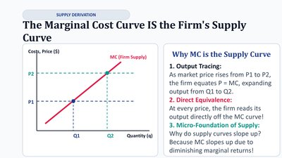
The Marginal Cost Curve IS the Firm's Supply Curve
Supply Derivation
Output Tracing: As price rises, the firm increases output along its MC curve.
Direct Equivalence: At every price, the firm reads its output directly off the MC curve.
Micro-Foundation: The MC curve slopes upward due to diminishing marginal returns.
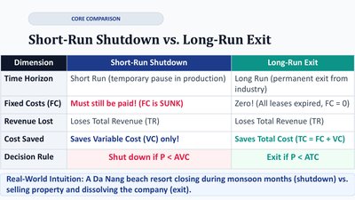
Short-Run Shutdown vs. Long-Run Exit
Core Comparison
Dimension | Short-Run Shutdown | Long-Run Exit |
|---|---|---|
Time Horizon | Short Run (temporary pause) | Long Run (permanent exit) |
Fixed Costs (FC) | Must still be paid (sunk) | Zero (all leases expired) |
Revenue Lost | Loses Total Revenue (TR) | Loses Total Revenue (TR) |
Cost Saved | Saves Variable Cost (VC) only | Saves Total Cost (TC = FC + VC) |
Decision Rule | Shut down if P < AVC | Exit if P < ATC |
Example: A beach resort closing for the monsoon (shutdown) vs. selling the property (exit).
The Short-Run Shutdown Rule & Sunk Costs
Concepts and Mathematical Proof
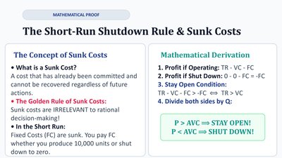
Sunk Costs: Costs already committed and unrecoverable; irrelevant to shutdown decisions.
Shutdown Rule: In the short run, shut down if .
Mathematical Derivation:
Profit if Operating:
Profit if Shut Down:
Stay Open Condition: or
Divide by Q: (Stay Open), (Shut Down)
The Competitive Firm's Short-Run Supply Curve
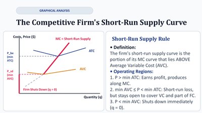
Short-Run Supply Rule
The firm's short-run supply curve is the portion of its MC curve above AVC.
Operating Regions:
P > min ATC: Earns profit, produces along MC.
min AVC < P < min ATC: Short-run loss, but covers VC and part of FC.
P < min AVC: Shuts down immediately (q = 0).
The Long-Run Entry and Exit Decision
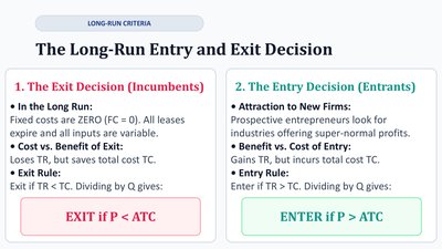
Entry and Exit Criteria
Exit Decision (Incumbents): Exit if (cannot cover total cost in the long run).
Entry Decision (Entrants): Enter if (can earn profit above total cost).
Measuring Profit and Loss Graphically
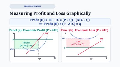
Profit Rectangles
Profit ():
Economic Profit:
Economic Loss:
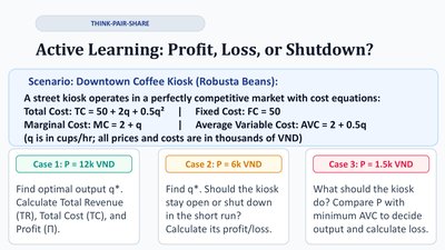
Active Learning: Profit, Loss, or Shutdown?
Scenario Analysis
A street kiosk operates in a perfectly competitive market with given cost equations. Students are asked to determine optimal output, profit/loss, and shutdown decisions under different price scenarios.
Case 1: P = 12k VND (Find optimal output, TR, TC, profit)
Case 2: P = 6k VND (Should the kiosk stay open or shut down?)
Case 3: P = 1.5k VND (Compare P with minimum AVC, calculate loss)
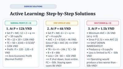
Active Learning: Step-by-Step Solutions
Worked Examples
Case 1 (Normal Profit): At P = 12k VND, profit is zero (normal profit).
Case 2 (Stay Open at Loss): At P = 6k VND, the kiosk should stay open since P > AVC, even though it incurs a loss.
Case 3 (Shut Down): At P = 1.5k VND, P < min AVC, so the kiosk should shut down immediately.
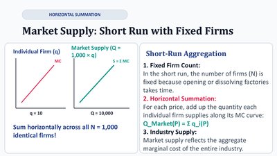
Market Supply: Short Run with Fixed Firms
Horizontal Summation
Fixed Firm Count: In the short run, the number of firms is fixed.
Horizontal Summation: Market supply is the sum of all individual firms' MC curves at each price.
Industry Supply: Reflects the aggregate marginal cost of the industry.
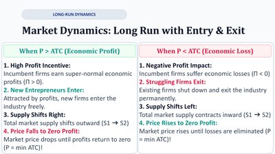
Market Dynamics: Long Run with Entry & Exit
Long-Run Dynamics
When P > ATC (Economic Profit):
Incumbent firms earn super-normal profits.
New firms enter, shifting supply right and driving price down to zero profit.
When P < ATC (Economic Loss):
Firms incur losses and exit the market.
Supply contracts, price rises until losses are eliminated.
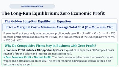
The Long-Run Equilibrium: Zero Economic Profit
Equilibrium Condition
Golden Long-Run Equilibrium Equation: ()
Firms earn zero economic profit (normal profit) in the long run due to free entry and exit.
Economic Profit Includes All Opportunity Costs: Zero economic profit means the firm covers all explicit and implicit costs, including the owner's opportunity cost.