뒤로
Firms in Perfectly Competitive Markets: Microeconomics Study Guide
스터디 가이드 - 스마트 노트
 자료에 맞춘 맞춤형 노트, 핵심 정의, 예시, 맥락을 확장해 제공합니다.
Firms in Perfectly Competitive Markets
Market Structures
Microeconomics classifies markets based on the number of firms, product differentiation, and ease of entry. Understanding these structures is essential for analyzing firm behavior and market outcomes.
Perfect Competition: Many firms, identical products, high ease of entry.
Monopolistic Competition: Many firms, differentiated products, high ease of entry.
Oligopoly: Few firms, identical or differentiated products, low ease of entry.
Monopoly: One firm, unique product, entry blocked.
Examples: Wheat farming and poultry farming are close to perfect competition; clothing stores and restaurants are monopolistic competition; streaming services and computer manufacturing are oligopolies; tap water and mail delivery are monopolies.
Perfectly Competitive Markets
A perfectly competitive market is characterized by many buyers and sellers, identical products, and no barriers to entry. Firms are price takers, meaning they cannot influence the market price.
Horizontal Demand Curve: Each firm faces a perfectly elastic demand at the market price.
Market Equilibrium: The collective actions of all firms and consumers determine the market price.
Example: Wheat farmers receive the same price per bushel regardless of their individual output.
Profit Maximization in Perfect Competition
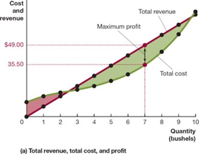
Firms aim to maximize profit, defined as total revenue minus total cost. In perfect competition, price equals both average revenue and marginal revenue.
Profit Formula:
Average Revenue (AR):
Marginal Revenue (MR):
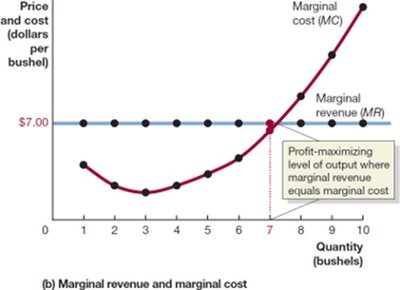
Profit Maximization Rule: Produce where (Marginal Cost).
For perfect competition:
Example: Farmer Parker maximizes profit at 7 bushels, where MR equals MC.
Illustrating Profit or Loss on the Cost Curve Graph
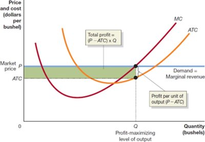
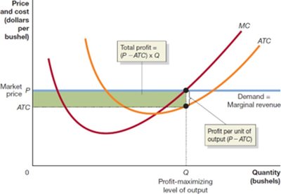
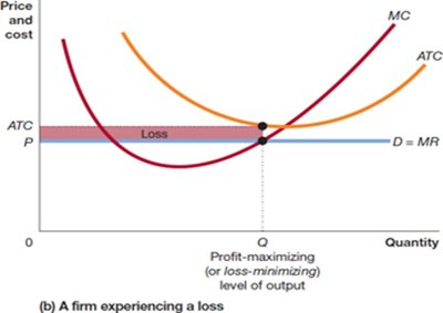
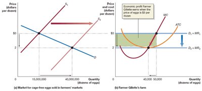
Profit or loss can be visualized using cost curves. The area between price and average total cost (ATC) at the profit-maximizing output represents total profit.
Profit per unit:
Total profit:
Break-Even and Loss-Minimizing Output
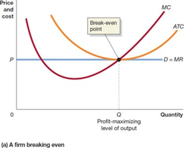
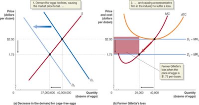
Even if a firm cannot make a profit, it should produce at the level where MC = MR to minimize losses. The break-even point occurs when price equals ATC.
Break-even:
Loss:
Profit:
Short-Run Production and Shutdown Decision
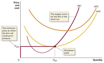
Firms may shut down temporarily if the price falls below average variable cost (AVC). Fixed costs are considered sunk and should not affect the shutdown decision.
Shutdown Rule: If , produce zero output.
Supply Curve: The firm's marginal cost curve above AVC is its supply curve in the short run.
Entry and Exit in the Long Run
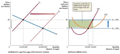
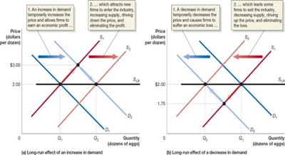
Economic profit attracts new firms, increasing supply and lowering price. Economic losses cause firms to exit, decreasing supply and raising price. In the long run, firms earn zero economic profit (break even).
Implicit Costs: Opportunity costs such as foregone salary and investment income must be included in total cost.
Long-Run Equilibrium: Entry and exit ensure price equals minimum ATC.
Explicit Costs | Implicit Costs | Total Cost |
|---|---|---|
Water: $10,000 Wages: $18,000 Fertilizer: $12,000 Electricity: $5,000 Bank loan: $10,000 | Forgone salary: $30,000 Investment opportunity cost: $5,000 | $90,000 |
Long-Run Supply Curve
In a perfectly competitive market, the long-run supply curve is horizontal at the minimum ATC. The number of firms adjusts to meet demand at this price.
Long-run supply curve: Shows the relationship between market price and quantity supplied in the long run.
Increasing-Cost and Decreasing-Cost Industries
Not all industries have constant costs. If new entrants face higher costs, the industry is increasing-cost and the long-run supply curve slopes upward. If costs fall as output increases, the industry is decreasing-cost and the supply curve slopes downward.
Increasing-cost industry: Upward-sloping long-run supply curve.
Decreasing-cost industry: Downward-sloping long-run supply curve.
Perfect Competition and Efficiency
Perfect competition leads to both productive and allocative efficiency.
Productive efficiency: Goods are produced at the lowest possible cost.
Allocative efficiency: Goods are produced up to the point where marginal benefit equals marginal cost.
Benchmark: These efficiencies are used to measure the performance of other market structures.
Applications and Real-World Examples
Case studies such as cage-free eggs and sneaker reselling illustrate how entry and exit affect profits and prices in competitive markets.