Models and Data

Introduction to Economic Models

Economic models are simplified representations of reality that help economists understand and predict economic phenomena. Models are essential tools for analyzing complex systems and making informed decisions.

• Model: A simplified description of reality used to explain and predict economic outcomes.

• Data: Empirical evidence used to evaluate the accuracy of models and understand how the world works.

• Correlation vs. Causality: Correlation does not imply causality; just because two variables move together does not mean one causes the other.

• Experiments: Help economists measure cause and effect relationships.

Example: Airplane Model

Models can take many forms, from mathematical equations to physical representations. For instance, a paper airplane is a model that simplifies the concept of flight, helping us understand aerodynamics without building a real airplane.

Additional info: The image illustrates how models (like a paper airplane) are simplified versions of reality (a real airplane), capturing essential features while omitting unnecessary complexity.

Evidence-Based Economics

Opportunity Cost of College

Economists use data to evaluate decisions, such as whether attending college is worth the cost. Opportunity cost is a key concept, representing the value of the next best alternative forgone.

• Tuition and Fees: Domestic and international students face different costs.

• Opportunity Cost: The minimum wage and hours spent in college represent income that could have been earned elsewhere.

• Calculation Example: Opportunity cost for a student working 50 hours/week at $17.60/hour for 28 weeks is $24,640.

The Scientific Method in Economics

Steps of the Scientific Method

The scientific method, also known as empiricism, is fundamental to economic analysis. It involves developing models and testing them with data.

• Step 1: Develop models that explain some part of the world.

• Step 2: Test those models using data to see how closely the model matches observed reality.

Case Study: The Wright Brothers

The Wright brothers succeeded in building a functional airplane by first testing models in a wind tunnel, demonstrating the importance of model testing before real-world application.

Returns to Education

Modeling Returns to Education

Economists often use models to estimate the returns to education, such as the increase in earnings associated with additional years of schooling.

• Assumption: Each additional year of education results in a 10% increase in future earnings.

• Example Calculation:

  • First year: $15 \times 1.10 = $16.50

  • Second year: $16.50 \times 1.10 = $18.15

  • Third year: $18.15 \times 1.10 = $19.965

  • Fourth year: $19.965 \times 1.10 = $21.9615

  • General formula:

• Percentage Increase: or 46.41%

• Model Prediction:

Variation and Testing Predictions

Models are not exact; they generate predictions that can be tested with data. The average can mask variation, and not everyone will see the same returns to education.

Empirical Data: Canadian Wages by Education Level

Example: College graduates earn 43.5% more than high school graduates, close to the model's prediction of 46%.

Mean, Median, and Variance

Understanding Measures of Central Tendency

Economists use statistical measures like the mean and median to summarize data. The mean is the average, while the median is the middle value.

• Mean: Sum of all observations divided by the number of observations.

• Median: The middle value in a sorted list of data.

• Variance: A measure of dispersion or inequality in the data.

Example: In three samples of five incomes, the median remains 50, but the mean changes depending on the distribution, highlighting differences in inequality.

Causation and Correlation

Distinguishing Causation from Correlation

It is crucial to distinguish between causation (one thing directly affects another) and correlation (two things are related). Not all correlations imply causality.

• Causation: Direct cause-and-effect relationship.

• Correlation: Statistical relationship between two variables.

• Types of Correlation:

  • Positive: Both variables move in the same direction.

  • Negative: Variables move in opposite directions.

  • Spurious: Statistical relationship without causal connection.

Spurious Correlation Examples

Spurious correlations are statistical relationships that do not reflect a true causal link. These can be misleading if interpreted as causation.

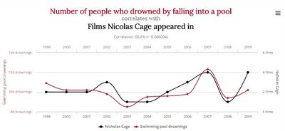
Additional info: These images show examples of spurious correlations, emphasizing the importance of careful interpretation of statistical relationships in economics.

Why Correlation Is Not Causality

• Omitted Variables: Ignoring relevant factors can lead to misleading correlations.

• Reverse Causality: The direction of cause and effect may be opposite to what is assumed.

Example: In studies about dairy cows, gambling seniors, or exercising seniors, omitted variables or reverse causality may explain observed correlations.

Experiments in Economics

Experiments help distinguish causality from correlation. Controlled experiments randomly assign subjects to treatment and control groups, while natural experiments rely on external events.

• Controlled Experiments: Researcher assigns groups.

• Natural Experiments: Groups are formed by external factors.

Example: The U.K. raising the minimum drop-out age in 1947 created a natural experiment to measure the effect of an extra year of schooling.

Appendix: Equations and Graphs

Graphing Functions

Economists use mathematical functions to model relationships between variables. The general form is:

• For demand and supply: and

• Linear example:

• Intercept (A): The value of Y when X = 0.

• Slope (B): , the rate at which Y changes with X.

Example: If and , then .

Practice Problems

Algebraic and Graphical Solutions

• Problem 1: Find two numbers whose sum is 385 and whose difference is 97.

• Problem 2: A fishing boat brings in cod and haddock. Cod sells for $2.00/lb, haddock for $1.50/lb. Total catch: 5,000 lbs, total revenue: $9,000. Find the pounds of each fish caught.

Additional info: These problems reinforce algebraic and graphical skills essential for microeconomic analysis.