뒤로
Monopoly: Market Power, Barriers, and Pricing Strategies
스터디 가이드 - 스마트 노트
 자료에 맞춘 맞춤형 노트, 핵심 정의, 예시, 맥락을 확장해 제공합니다.
Monopoly: Market Power Foundations
What is a Monopoly?
A monopoly is a market structure where a single firm is the sole seller of a product without close substitutes. Unlike competitive firms, a monopoly is a price-maker, meaning it has the power to set and influence the price of its product. The essential source of monopoly power is the presence of barriers to entry, which prevent other firms from entering the market and competing away profits.
Monopoly: Sole seller, no close substitutes.
Price-Maker: Sets price, does not take it as given.
Barriers to Entry: Fundamental cause of monopoly power.
Competitive Firm: Price-taker, faces horizontal demand (P = MR).
Monopoly Firm: Price-maker, faces downward-sloping demand (MR < P).
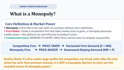
Reality Check: Large profits alone do not indicate a monopoly; barriers to entry are essential.
Structural Sources: The Three Major Barriers to Entry
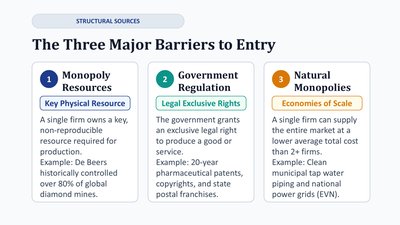
1. Monopoly Resources
Key Physical Resource: A single firm controls a vital, non-reproducible resource (e.g., De Beers and diamonds).
2. Government Regulation
Legal Exclusive Rights: Government grants exclusive rights (e.g., patents, copyrights, franchises).
3. Natural Monopolies
Economies of Scale: One firm can supply the market at a lower average cost than multiple firms (e.g., utilities).
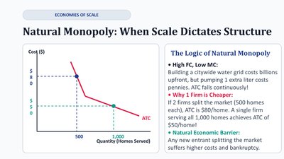
Economies of Scale: Natural Monopoly
Natural Monopoly: When Scale Dictates Structure
A natural monopoly arises when a single firm can supply the entire market at a lower average total cost (ATC) than multiple firms due to high fixed costs and low marginal costs. This creates a natural economic barrier to entry, as new entrants would face higher costs and likely fail.
High Fixed Costs, Low Marginal Costs: Infrastructure-heavy industries (e.g., water supply).
Why One Firm is Cheaper: Spreading fixed costs over more units lowers ATC.
Natural Economic Barrier: New entrants splitting the market face higher costs and risk bankruptcy.
Demand Contrast: Competitive Firm vs. Monopolist
Demand Curves
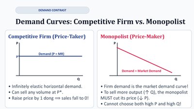
Competitive Firm (Price-Taker): Faces a perfectly elastic (horizontal) demand curve at market price (P = MR).
Monopolist (Price-Maker): Faces the market demand curve, which is downward sloping. To sell more, the monopolist must lower the price, and cannot choose both price and quantity independently.
Revenue Dynamics: Marginal Revenue and Price
Why Marginal Revenue is ALWAYS Less Than Price
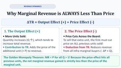
For a monopolist, marginal revenue (MR) is always less than price (P) for all quantities greater than one. This is because selling an additional unit requires lowering the price on all units sold, not just the marginal unit.
Output Effect (+): Selling more increases total revenue.
Price Effect (–): Lowering price reduces revenue from all previous units.
Golden Monopoly Theorem: for all .
Monopoly Revenue Schedule: Active Learning Example
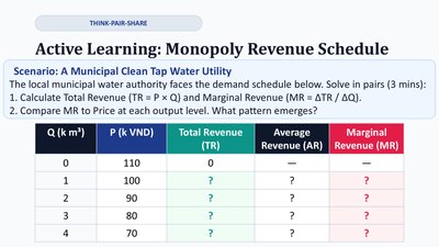
Scenario: Municipal Clean Tap Water Utility
Given a demand schedule, students calculate Total Revenue (TR) and Marginal Revenue (MR) at each output level, observing that MR falls faster than price.
Q (k m3) | P (k VND) | Total Revenue (TR) | Average Revenue (AR) | Marginal Revenue (MR) |
|---|---|---|---|---|
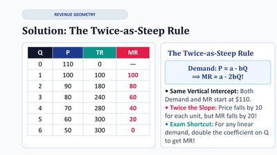
0 | 110 | 0 | - | - |
1 | 100 | 100 | 100 | 100 |
2 | 90 | 180 | 90 | 80 |
3 | 80 | 240 | 80 | 60 |
4 | 70 | 280 | 70 | 40 |
5 | 60 | 300 | 60 | 20 |
Revenue Geometry: The Twice-as-Steep Rule
Solution: The Twice-as-Steep Rule
For a linear demand curve , the marginal revenue curve is . The MR curve shares the same vertical intercept as demand but is twice as steep.
Exam Shortcut: For linear demand, double the coefficient on Q to get MR.
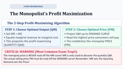
2-Step Decision Rule: The Monopolist's Profit Maximization
The 2-Step Profit-Maximizing Algorithm
Choose Optimal Output (QM): Set MR = MC to find the profit-maximizing quantity.
Choose Optimal Price (PM): Project QM up to the demand curve to find the highest price consumers will pay.
Critical Warning: The monopoly price is never read off the MR curve; it must be read from the demand curve after finding QM.
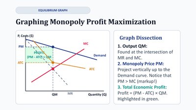
Equilibrium Graph: Graphing Monopoly Profit Maximization
Graph Dissection
Output (QM): Intersection of MR and MC.
Monopoly Price (PM): Project QM up to the demand curve (PM > MC).
Total Economic Profit:
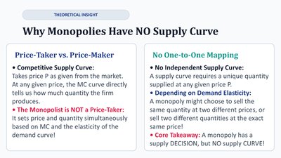
Theoretical Insight: Why Monopolies Have NO Supply Curve
Price-Taker vs. Price-Maker
Competitive Supply Curve: MC curve tells us how much the firm produces at each price.
Monopolist: Sets price and quantity simultaneously; no unique supply curve.
No One-to-One Mapping
No Independent Supply Curve: Quantity supplied depends on demand elasticity; a monopoly can supply different quantities at the same price or the same quantity at different prices.
Core Takeaway: Monopoly has a supply decision, but no supply curve.
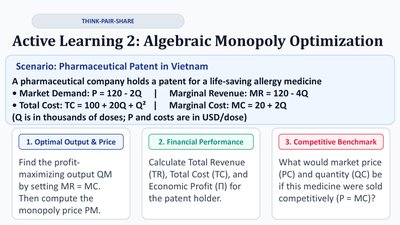
Active Learning 2: Algebraic Monopoly Optimization
Scenario: Pharmaceutical Patent in Vietnam
Market Demand:
Marginal Revenue:
Total Cost:
Marginal Cost:
Find profit-maximizing output (QM) by setting MR = MC, then compute monopoly price (PM).
Calculate Total Revenue (TR), Total Cost (TC), and Economic Profit.
Find competitive price (PC) and quantity (QC) where P = MC.
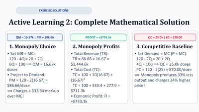
Exercise Solutions: Complete Mathematical Solution
Monopoly Choice: ,
Monopoly Profits: , , Economic Profit =
Competitive Baseline: ,
Welfare Loss: The Welfare Cost of Monopoly (Deadweight Loss)
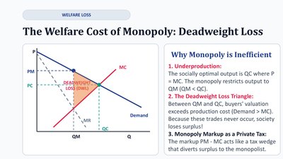
Why Monopoly is Inefficient
Underproduction: Monopoly restricts output below the socially optimal level (where P = MC).
Deadweight Loss Triangle: The area between QM and QC, where buyers' valuation exceeds production cost, represents lost societal welfare.
Monopoly Markup: The difference PM - MC acts like a private tax.
Patent Dynamics: Case Study—Monopoly vs. Generic Drugs
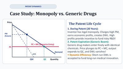
The Patent Life Cycle
During Patent: Inventor has legal monopoly, charges high price, earns economic profits, and creates deadweight loss (DWL).
Patent Expiration: Generic entry drives price to competitive level (P = MC), output expands, and DWL vanishes.
Dynamic Efficiency: Short-run DWL is accepted to fund long-run innovation.
Pricing Strategies: Price Discrimination
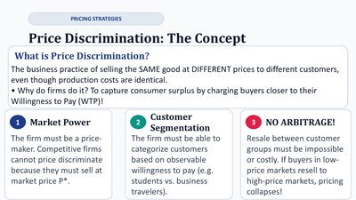
What is Price Discrimination?
Price discrimination is the practice of selling the same good at different prices to different customers, even though production costs are identical. Firms do this to capture more consumer surplus by charging buyers closer to their willingness to pay (WTP).
Market Power: Only price-makers can price discriminate.
Customer Segmentation: Firms must be able to categorize customers based on observable traits.
No Arbitrage: Resale between customer groups must be impossible or costly.
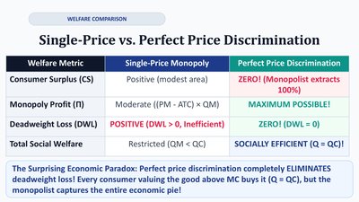
Welfare Comparison: Single-Price vs. Perfect Price Discrimination
Welfare Metric | Single-Price Monopoly | Perfect Price Discrimination |
|---|---|---|
Consumer Surplus (CS) | Positive (modest area) | ZERO! (Monopolist extracts 100%) |
Monopoly Profit (π) | Moderate | MAXIMUM POSSIBLE! |
Deadweight Loss (DWL) | POSITIVE (DWL > 0, Inefficient) | ZERO! (DWL = 0) |
Total Social Welfare | Restricted (QM < QC) | SOCIALLY EFFICIENT (Q = QC!) |
Economic Paradox: Perfect price discrimination eliminates deadweight loss, but the monopolist captures all surplus.
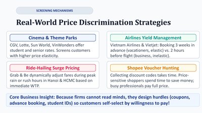
Screening Mechanisms: Real-World Price Discrimination Strategies
Cinema & Theme Parks: Student and senior rates segment by elasticity.
Airlines Yield Management: Advance booking discounts for elastic travelers.
Ride-Hailing Surge Pricing: Dynamic pricing during peak demand.
Shopee Voucher Hunting: Discounts for price-sensitive shoppers.
Core Business Insight: Firms design hurdles (coupons, advance booking, student IDs) so customers self-select by willingness to pay.