뒤로
The Theory of Consumer Choice: Budget Constraints, Indifference Curves, and the Microfoundations of Demand
스터디 가이드 - 스마트 노트
 자료에 맞춘 맞춤형 노트, 핵심 정의, 예시, 맥락을 확장해 제공합니다.
The Theory of Consumer Choice
Introduction
The theory of consumer choice explores how individuals allocate their limited income among various goods and services to maximize their satisfaction. This topic forms the microeconomic foundation for understanding demand, market behavior, and consumer welfare.
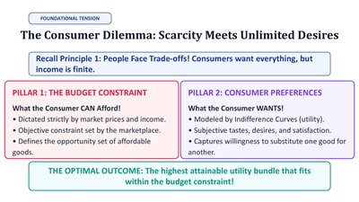
The Consumer Dilemma: Scarcity Meets Unlimited Desires
Foundational Principles
Scarcity vs. Unlimited Wants: Consumers face trade-offs because their desires exceed their financial resources.
Pillar 1: The Budget Constraint
Represents what a consumer can afford, dictated by market prices and income.
Defines the opportunity set of affordable goods.
Pillar 2: Consumer Preferences
Represents what a consumer wants, modeled by indifference curves (utility).
Captures willingness to substitute one good for another.
Optimal Outcome: The highest attainable utility bundle that fits within the budget constraint.
The Budget Constraint: Mathematical Formulation
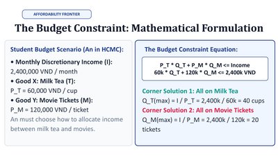
Budget Equation and Example
Budget Constraint Equation:
Example: Student in Ho Chi Minh City with 2,400,000 VND/month, choosing between milk tea (60,000 VND/cup) and movie tickets (120,000 VND/ticket).
Corner Solutions:
All income on milk tea: cups
All income on movies: tickets
Graphing the Budget Line & Market Opportunity Cost
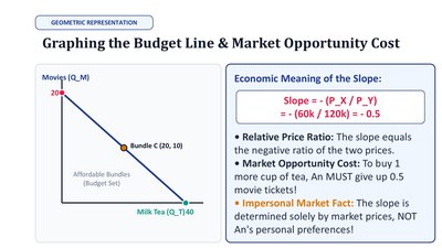
Budget Line and Slope
Budget Line: Shows all combinations of two goods a consumer can afford.
Slope of Budget Line:
Economic Meaning: The slope represents the opportunity cost of one good in terms of the other (e.g., to buy one more cup of tea, must give up 0.5 movie tickets).
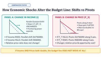
How Economic Shocks Alter the Budget Line: Shifts vs. Pivots
Comparative Statics
Change in Income: Parallel shift of the budget line (outward if income rises, inward if income falls). Slope unchanged.
Change in Price: Pivot of the budget line around one axis. Slope changes, altering the opportunity cost.
Simultaneous Change: If both income and prices double, the budget line does not move.
Preferences & Indifference Curves: What the Consumer Wants
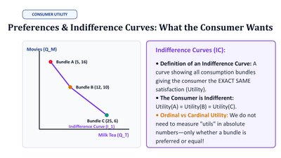
Indifference Curves (IC)
Definition: A curve showing all consumption bundles that give the consumer the same level of satisfaction (utility).
Indifference: The consumer is equally happy with any bundle on the same curve.
Ordinal Utility: Only the order of preferences matters, not the absolute value of utility.
The Marginal Rate of Substitution (MRS)
Definition and Diminishing MRS
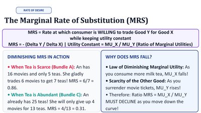
MRS: The rate at which a consumer is willing to trade Good Y for Good X while keeping utility constant.
Formula:
Diminishing MRS: As a consumer has more of Good X, they are willing to give up less of Good Y for additional units of X.
Law of Diminishing Marginal Utility: Marginal utility of a good decreases as its quantity increases.
The Four Axiomatic Properties of Indifference Curves
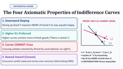
Properties
Downward Sloping: Giving up one good requires more of the other to maintain utility.
Higher ICs Preferred: Higher curves represent more of both goods.
Curves Cannot Cross: Crossing would violate transitivity of preferences.
Bowed Inward (Convex): Consumers prefer balanced bundles due to diminishing MRS.
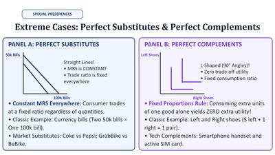
Extreme Cases: Perfect Substitutes & Perfect Complements
Special Preferences
Perfect Substitutes: Straight-line ICs, constant MRS. Example: Different denominations of currency.
Perfect Complements: L-shaped ICs, fixed consumption ratio. Example: Left and right shoes, smartphone and SIM card.
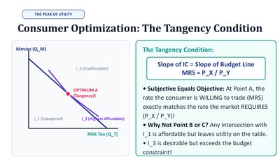
Consumer Optimization: The Tangency Condition
Utility Maximization
Tangency Condition: The optimal bundle occurs where the slope of the indifference curve equals the slope of the budget line.
Mathematically:
Interpretation: The rate at which the consumer is willing to trade matches the market rate.
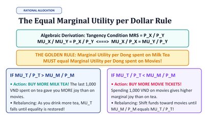
The Equal Marginal Utility per Dollar Rule
Rational Allocation
Rule: Marginal utility per unit of currency spent should be equal across all goods for utility maximization.
Formula:
Adjustment: If , buy more of X and less of Y until equality is restored.
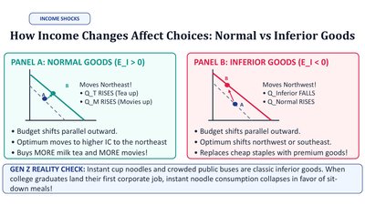
How Income Changes Affect Choices: Normal vs Inferior Goods
Income Effects
Normal Goods: Demand increases as income rises (budget line shifts outward, higher IC chosen).
Inferior Goods: Demand decreases as income rises (budget line shifts outward, but consumer buys less of the inferior good).
Example: Instant noodles as an inferior good for college students.
Decomposing a Price Drop: Substitution vs Income Effects
Analytical Decomposition
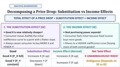
Total Effect: Price drop = Substitution Effect + Income Effect
Substitution Effect: Good X is relatively cheaper; consumer moves along the IC to buy more X, fewer Y.
Income Effect: Real purchasing power expands; consumer moves to a higher IC, buying more of both goods if normal.
Good | Substitution Effect | Income Effect (Normal) | Net Total Effect |
|---|---|---|---|
Good X (P_X fell) | Increases (X up) | Increases (X up) | UNAMBIGUOUSLY RISES! |
Good Y (P_Y constant) | Decreases (Y down) | Increases (Y up) | Ambiguous (Depends on SE vs IE) |
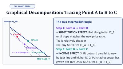
Graphical Decomposition: Tracing Point A to B to C
The Two-Step Walkthrough
Step 1 (A to B): Substitution effect—move along the initial IC as the price ratio changes.
Step 2 (B to C): Income effect—shift to a higher IC as purchasing power increases.
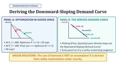
Deriving the Downward-Sloping Demand Curve
Microfoundation of Demand
Optimization in Goods Space: Each price-quantity pair on the demand curve corresponds to a utility-maximizing choice.
Law of Demand: The downward slope is derived from utility maximization, not assumed.
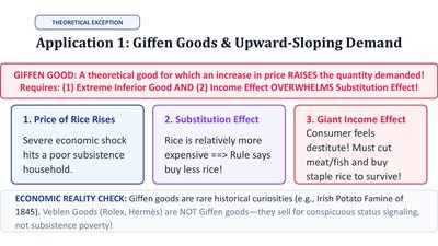
Application 1: Giffen Goods & Upward-Sloping Demand
Theoretical Exception
Giffen Good: A good for which an increase in price raises the quantity demanded, due to a strong negative income effect overwhelming the substitution effect.
Conditions: Must be an extreme inferior good with a large income effect.
Example: Historical cases like the Irish Potato Famine.
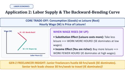
Application 2: Labor Supply & The Backward-Bending Curve
Labor-Leisure Trade-Off
Core Trade-Off: Consumption (goods) vs. leisure (rest); wage is the price of leisure.
When Wage Rises:
Substitution Effect: Leisure is more expensive, so work more hours (dominates at low wages).
Income Effect: Higher income allows more leisure, so work fewer hours (dominates at high wages).
Result: Labor supply curve may bend backward at high wage levels.