Acceleration and Kinematic Graphs

Introduction to Acceleration

Acceleration is a fundamental concept in kinematics, describing how the velocity of an object changes with time. Understanding acceleration is essential for analyzing motion in physics, especially when using calculus-based approaches.

• Position (x): The location of an object along a coordinate axis, typically measured from an origin.

• Velocity (v): The rate of change of position with respect to time. It can be positive or negative, indicating direction.

• Acceleration (a): The rate of change of velocity with respect to time. It can also be positive or negative, depending on the direction of the change.

• Jerk: The rate of change of acceleration (not typically used in introductory courses).

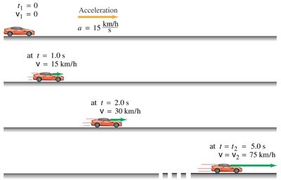
Example: If a car's velocity increases by 15 km/h every second, its acceleration is +15 (km/h)/s.

Constant Acceleration

When acceleration is constant, the velocity of an object changes linearly with time. This is a common scenario in introductory physics problems.

• For constant acceleration a, the velocity at time t is given by:

• Where v_0 is the initial velocity.

• For each second, the velocity increases (or decreases) by the value of the acceleration.

Example: If a car starts from rest and accelerates at 15 km/h per second, after 1 second its velocity is 15 km/h, after 2 seconds it is 30 km/h, and after 5 seconds it is 75 km/h.

Negative Acceleration (Deceleration)

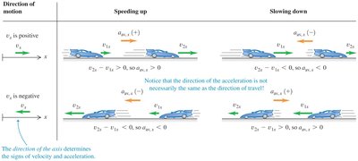
Negative acceleration, often called deceleration, occurs when the acceleration vector is opposite to the velocity vector, causing the object to slow down. However, deceleration is not always the same as negative acceleration; it depends on the direction of motion and the chosen coordinate system.

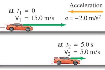
• For negative acceleration (e.g., a = -2.0 m/s2), the velocity decreases by 2.0 m/s every second.

• Deceleration means the speed is decreasing, but the sign of acceleration depends on the coordinate system.

Example: A car moving at 15.0 m/s slows down to 5.0 m/s in 5.0 seconds with an acceleration of -2.0 m/s2.

Mathematical Definitions Using Calculus

Calculus provides precise definitions for velocity and acceleration:

• Average velocity:

• Instantaneous velocity:

• Average acceleration:

• Instantaneous acceleration:

Signs of Velocity and Acceleration

The signs of velocity and acceleration depend on the chosen coordinate system and the direction of motion. Positive and negative signs indicate direction, not just increase or decrease in speed.

• If velocity and acceleration have the same sign, the object speeds up.

• If velocity and acceleration have opposite signs, the object slows down (decelerates).

Graphical Interpretation of Acceleration

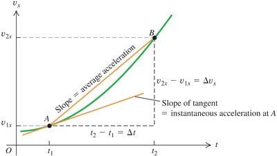
Acceleration can be interpreted as the slope of the velocity vs. time graph. The average acceleration over a time interval is the slope of the secant line, while the instantaneous acceleration at a point is the slope of the tangent line.

• Average acceleration:

• Instantaneous acceleration:

Kinematic Graphing Relationships

Understanding the relationships between position, velocity, and acceleration graphs is crucial for analyzing motion:

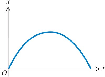
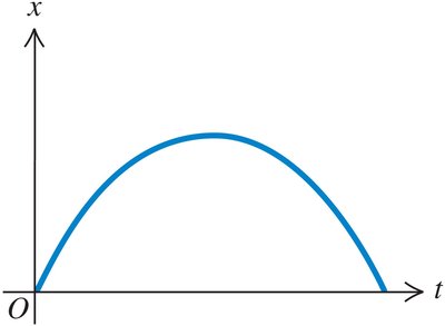
• At any time t, velocity v(t) is the slope of the position vs. time (x vs. t) graph.

• Over any interval Δt, displacement Δx is the net area under the velocity vs. time (v vs. t) graph.

• At any time t, acceleration a(t) is the slope of the velocity vs. time (v vs. t) graph.

• Over any interval Δt, change in velocity Δv is the net area under the acceleration vs. time (a vs. t) graph.

These relationships allow for the graphical analysis of motion, even without explicit equations.

Review Quiz: Interpreting Kinematic Graphs

Students are often asked to interpret position vs. time and velocity vs. time graphs. Key questions include identifying when an object is at rest, when it reverses direction, and how its speed and acceleration change over time.

• Example: Given a velocity vs. time graph, determine at which points the object is at rest (v = 0), when it changes direction (velocity changes sign), and when it is speeding up or slowing down (compare signs of v and a).

Summary Table: Kinematic Quantities and Their Graphical Relationships

Additional info: In PHYS 151, calculus is introduced for definitions, but most problems use algebraic methods for constant acceleration. The concept of jerk is mentioned for completeness but not used in this course.