Free Fall: Measuring g Using the Spark Timer Apparatus

Introduction to Free Fall Experiments

Free fall experiments are fundamental in physics for understanding motion under constant acceleration due to gravity. In this lab, a mass attached to thermal paper is dropped, and a spark timer marks the paper at regular intervals, creating a motion diagram. The experiment aims to analyze the kinematic equations for free fall and determine the local acceleration due to gravity, g, using graphical and tabular analysis in Excel.

Experimental Apparatus and Setup

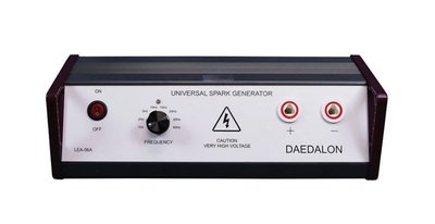
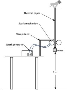
The experiment utilizes a spark generator and a spark mechanism to mark the thermal paper as the mass falls. The generator operates at 60 Hz, ensuring consistent time intervals between marks. The setup includes a clamp stand, thermal paper, and a mass (≥200 g), positioned about 1 meter above the ground.

• Spark Generator: Provides high voltage pulses to mark the paper at regular intervals.

• Thermal Paper: Records the position of the mass at each time interval.

• Clamp Stand: Holds the spark mechanism and paper vertically.

• Mass: Attached to the paper, falls freely under gravity.

Theory: Kinematics of Free Fall

Position vs. Time Relationship

For an object in free fall with constant acceleration g (downwards), the position as a function of time is given by:

Where:

• y(t): Position at time t

• y_i: Initial position

• v_{y,i}: Initial velocity

• g: Acceleration due to gravity

Excel curve-fitting yields a quadratic equation of the form:

By comparing coefficients, the value of g can be extracted from the quadratic term.

Velocity vs. Time Relationship

Velocity is calculated as the average between two position points:

The corresponding time is the average of the two times:

For free fall, velocity as a function of time is:

This relationship is linear, and the slope of the velocity vs. time graph gives -g:

Thus, where m is the slope.

Data Analysis and Graphical Methods

Curve-Fitting and Extraction of g

Position vs. time data is plotted and fitted with a quadratic curve. The coefficient of the quadratic term is used to calculate the experimental value of g. Similarly, velocity vs. time data is plotted and fitted with a linear curve, and the slope provides another measure of g.

Uncertainty and Error Propagation

Measurement uncertainties are crucial for accurate data analysis. The rules for propagating uncertainties are:

• Add/Subtract: Add absolute uncertainties.

• Multiply/Divide: Add fractional uncertainties.

For example, for displacement:

For velocity:

Lab Procedure Overview

• Set up the apparatus as shown in the diagram.

• Attach the mass and thread the thermal paper through the spark mechanism.

• Operate the spark generator at 60 Hz and drop the mass.

• Record positions of the dots and analyze data in Excel.

Data Presentation and Reporting Guidelines

• Include units and uncertainties with all data.

• Present data tables and graphs with clear titles, axis labels, and error bars.

• Fit appropriate curves and report equations and uncertainties.

• Summarize results, discuss precision and accuracy, and identify sources of error.

Example Data Table Structure

Example Uncertainty Calculation Table

Summary of Key Concepts

• Free Fall: Motion under constant acceleration due to gravity.

• Kinematic Equations: Used to relate position, velocity, and acceleration.

• Graphical Analysis: Curve-fitting to extract physical parameters.

• Uncertainty: Essential for evaluating precision and accuracy.

Example: If the quadratic coefficient from Excel is -4.2553, then (additional info: actual calculation may require unit conversion and sign convention check).

Additional info: The experiment is directly relevant to kinematics, Newton's laws, and measurement/estimation topics in introductory college physics with calculus.