Motion Diagrams and Kinematic Quantities

Introduction to Motion Diagrams

Motion diagrams are visual tools used to represent the position of an object at successive time intervals. They help in understanding how an object's position changes over time and are foundational for analyzing motion in physics.

• Position: The location of an object at a particular instant, usually measured relative to a chosen origin.

• Displacement: The change in position of an object, a vector quantity.

• Velocity: The rate of change of position with respect to time, including direction (vector).

• Speed: The magnitude of velocity, a scalar quantity.

• Acceleration: The rate of change of velocity with respect to time (vector).

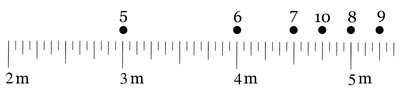
Example: A mouse drops a piece of cheese every second as it moves along a straight line. The positions of the cheese pieces indicate the mouse's position at each second, forming a motion diagram.

1D Motion: Position, Velocity, and Acceleration

Key Kinematic Quantities

In one-dimensional (1D) motion, the following quantities are essential for describing and analyzing motion:

Example: If a mouse moves from 3 m to 5 m in 2 seconds, its average velocity is \( \frac{5\,\text{m} - 3\,\text{m}}{2\,\text{s}} = 1\,\text{m/s} \).

Kinematic Equations for Constant Acceleration

Equations of Motion

When an object moves with constant acceleration, its position and velocity as functions of time can be described by the kinematic equations. These equations are derived using calculus and are fundamental for solving problems in 1D motion.

• First Equation (Velocity as a function of time):

• Second Equation (Position as a function of time):

• Third Equation (Velocity as a function of displacement):

Where:

• \( x_0 \): Initial position

• \( v_0 \): Initial velocity

• \( a \): Constant acceleration

• \( t \): Time elapsed

Example: A motorcycle accelerates from rest (\( v_0 = 0 \)) at \( 4.0\,\text{m/s}^2 \) until it travels 50 m. To find the time to reach 50 m:

• Use with , , , .

Instantaneous vs. Average Quantities

Definitions and Differences

It is important to distinguish between average and instantaneous quantities in kinematics:

• Average velocity:

• Instantaneous velocity:

• Average acceleration:

• Instantaneous acceleration:

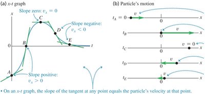
Example: The slope of the tangent to a position-time graph at any point gives the instantaneous velocity at that point.

Analyzing Motion with Diagrams and Graphs

Interpreting Motion Diagrams

Motion diagrams and graphs are used to determine the direction and magnitude of velocity and acceleration at different points in time. The sign of velocity and acceleration can be inferred from the spacing and direction of dots or from the slope of graphs.

• If acceleration is positive and velocity is positive, the object speeds up in the positive direction.

• If acceleration is negative and velocity is positive, the object slows down.

• If acceleration is positive and velocity is negative, the object slows down in the negative direction.

• If acceleration is negative and velocity is negative, the object speeds up in the negative direction.

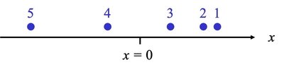
Example: In a motion diagram, if the dots get closer together, the object is slowing down; if they get farther apart, the object is speeding up.

Summary Table: 1D Kinematic Quantities

Additional info: The concepts and equations above are foundational for all subsequent topics in mechanics, including two-dimensional motion, Newton's laws, and energy analysis.