One-Dimensional Kinematics

Position, Displacement, and Distance

To analyze the motion of an object in one dimension, we first establish a coordinate system, typically an x-axis with a defined origin and positive direction. This allows us to describe the location and movement of objects quantitatively.

• Position (x): The location of an object relative to the origin of a coordinate system. The SI unit is the meter (m). Position is a vector quantity, meaning it has both magnitude and direction.

• Displacement (\( \Delta x \)): The change in position of an object, defined as the final position minus the initial position. Displacement is also a vector and can be positive or negative depending on direction. \[ \Delta x = x_f - x_i \]

• Distance: The total length of the path traveled, regardless of direction. Distance is a scalar quantity and always positive.

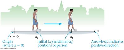
Additional info: In higher dimensions, displacement is represented as a vector difference using unit vectors in each direction.

Worked Examples: Displacement and Distance

Examples help clarify the distinction between displacement and distance:

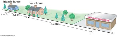
• Example 1: Walking from your house to a friend's house 2.1 miles away (negative x-direction). - Initial position: \( x_i = 0 \) - Final position: \( x_f = -2.1 \) mi - Displacement: \( \Delta x = -2.1 \) mi - Distance: 2.1 mi

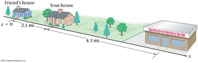
• Example 2: Walking from your house to the grocery store (4.3 mi), then returning home. - Initial position: \( x_i = 0 \) mi - Final position: \( x_f = 0 \) mi - Displacement: \( \Delta x = 0 \) mi - Distance: 8.6 mi (4.3 mi each way)

Average Speed and Average Velocity

To quantify how fast an object moves, we use average speed and average velocity:

• Average Velocity (\( v_{av} \)): Displacement divided by elapsed time. It is a vector and can be positive or negative. \[ v_{av} = \frac{\Delta x}{\Delta t} = \frac{x_f - x_i}{t_f - t_i} \]

• Average Speed: Distance divided by elapsed time. It is always positive and a scalar. \[ \text{Average Speed} = \frac{\text{Distance}}{\Delta t} \]

• Direction: For one-dimensional motion, the sign of average velocity indicates direction (positive for right, negative for left).

Position-Time Graphs and Average Velocity

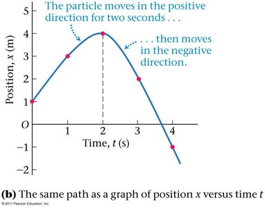
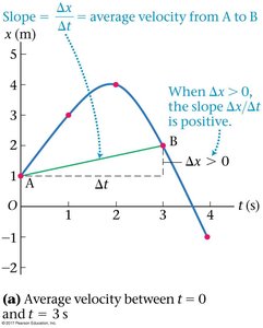
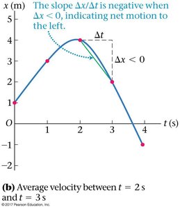
The slope of a line connecting two points on a position vs. time graph represents the average velocity over that interval. Tabulated data and graphs help visualize this relationship.

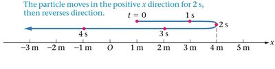
• Example: Average velocity between \( t = 0 \) s and \( t = 3 \) s: \[ v_{av} = \frac{2\,\text{m} - 1\,\text{m}}{3\,\text{s} - 0\,\text{s}} = 0.33\,\text{m/s} \]

• Example: Average velocity between \( t = 2 \) s and \( t = 3 \) s: \[ v_{av} = \frac{2\,\text{m} - 4\,\text{m}}{3\,\text{s} - 2\,\text{s}} = -2\,\text{m/s} \]

Instantaneous Velocity

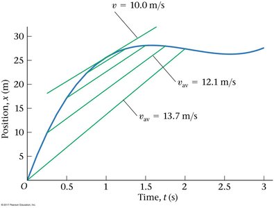
Instantaneous velocity is the velocity of an object at a specific instant. It is defined as the limit of the average velocity as the time interval approaches zero:

• Instantaneous Velocity (v): \[ v = \lim_{\Delta t \to 0} \frac{\Delta x}{\Delta t} \]

• The instantaneous velocity at a given time is the slope of the tangent line to the position vs. time graph at that point.

• Instantaneous Speed: The magnitude of the instantaneous velocity (always positive).

Acceleration

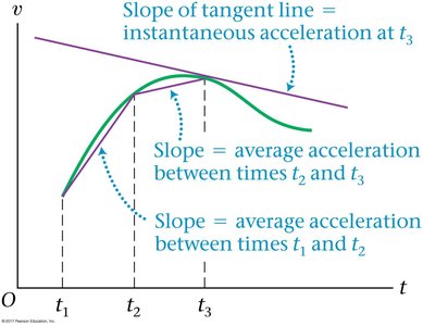
Acceleration measures how quickly velocity changes with time. Like velocity, it can be average or instantaneous:

• Average Acceleration (\( a_{av} \)): \[ a_{av} = \frac{\Delta v}{\Delta t} = \frac{v_f - v_i}{t_f - t_i} \]

• Instantaneous Acceleration (a): \[ a = \lim_{\Delta t \to 0} \frac{\Delta v}{\Delta t} \]

• SI unit: meter per second squared (m/s2).

Worked Example: Calculating Average Acceleration

Example: An electric sportscar accelerates from rest to 100 km/h in 2.6 s. What is its average acceleration in SI units?

• First, convert 100 km/h to m/s: \[ 100\,\text{km/h} = 27.8\,\text{m/s} \]

• Average acceleration: \[ a_{av} = \frac{27.8\,\text{m/s} - 0\,\text{m/s}}{2.6\,\text{s} - 0\,\text{s}} = 10.7\,\text{m/s}^2 \]

Additional info: Acceleration is a vector; its sign indicates direction (positive for acceleration in the positive x-direction, negative for the opposite).