Exponential Functions

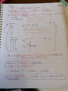
Definition and Properties

Exponential functions are a fundamental class of functions in precalculus, defined by the equation , where a is a constant and b is the base. These functions model rapid growth or decay and are continuous curves.

• Base (b): The number raised to the power of x. If , the function grows; if , the function decays.

• Exponent (x): The variable in the exponent determines the rate of change.

• Domain: All real numbers ().

• Range: All positive real numbers ().

• Intercept: The y-intercept occurs at , so .

• Negative Exponents: , which reflects the function across the y-axis.

Example: is an exponential growth function.

Characteristics of Exponential Functions

• Passes through the point (0, a).

• Asymptote at (the function never touches the x-axis).

• For , the graph rises rapidly to the right.

• For , the graph falls rapidly to the right.

• Domain is all real numbers; range is .

Example: grows faster than .

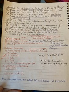
Interest Formulas

Exponential functions are used in financial mathematics to model compound interest.

• Simple Interest:

• Compound Interest:

• Continuous Compounding:

Example: If , , , , then .

Transformations of Exponential Functions

Types of Transformations

Exponential functions can be transformed using shifts, reflections, and stretches. These transformations alter the graph's position and shape.

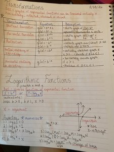
Logarithmic Functions

Definition and Properties

Logarithmic functions are the inverse of exponential functions. The logarithm base b of x, written as , answers the question: "To what exponent must b be raised to produce x?"

• Domain:

• Range: All real numbers

• Base (b): ,

• x-intercept: Occurs at

Example: is the inverse of .

Types of Logarithms

• Common Logarithm: , often written as

• Natural Logarithm: , written as

Example: is the natural logarithm of 2.

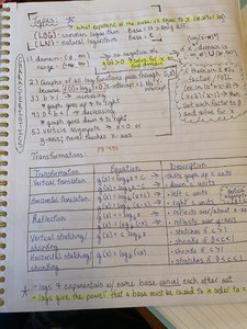
Transformations of Logarithmic Functions

Logarithmic functions can be transformed similarly to exponential functions.

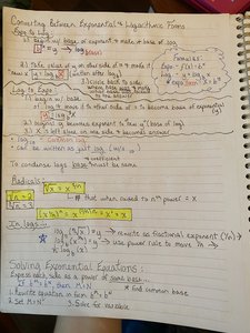
Converting Between Exponential and Logarithmic Forms

Exponential to Logarithmic

To convert an exponential equation to logarithmic form, use the definition: .

• Example:

Logarithmic to Exponential

To convert a logarithmic equation to exponential form, use: .

• Example:

Solving Exponential and Logarithmic Equations

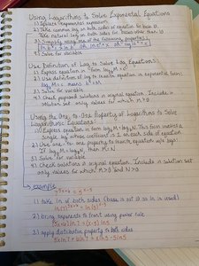
Solving Exponential Equations

To solve exponential equations, isolate the exponential expression and use logarithms if necessary.

1. Isolate the exponential term.

2. Take the logarithm of both sides (common or natural log).

3. Solve for the variable.

Example:

Solving Logarithmic Equations

To solve logarithmic equations, use properties of logarithms to combine or expand, then convert to exponential form.

1. Express logarithms in terms of a single log if possible.

2. Convert to exponential form.

3. Solve for the variable.

Example:

Exponential Growth and Decay; Modeling Data

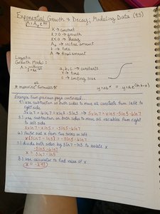
Exponential Growth and Decay Models

Exponential growth and decay describe processes where quantities increase or decrease at rates proportional to their current value. The general model is , where is the initial amount, is the growth (or decay) constant, and is time.

• Growth:

• Decay:

• Applications: Population growth, radioactive decay, financial investments

Example: If , , , then .

Logistic Growth Models

Logistic growth models describe situations where growth is limited by carrying capacity. The model is .

• a: Maximum value (carrying capacity)

• b: Constant related to initial value

• k: Growth rate

Example: Population growth in a limited environment.