Exponential Growth and Decay: Modeling

Exponential Models

Exponential models are used to describe processes that increase or decrease at rates proportional to their current value. The general form for exponential growth or decay is:

• Formula: , where:

  • = amount at time

  • = initial amount (when )

  • = growth () or decay () constant

  • = time (with )

• If , the function models exponential growth (e.g., population growth).

• If , the function models exponential decay (e.g., radioactive decay).

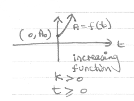
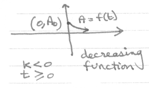
Key Properties:

• At , (since ).

• Exponential growth functions increase without bound as increases.

• Exponential decay functions approach zero as increases but never reach it.

Example 1: Population Growth

Suppose the population of Africa was 643 million in 1990 and 813 million in 2000. To model this with an exponential function:

• Let be years after 1990, so .

• Model:

• When , .

• Solving for :

• Model:

• To find when :

  • years after 1990 (i.e., by 2090)

Example 2: Carbon-14 Dating (Decay)

Carbon-14 decays exponentially with a half-life of about 5715 years. The half-life is the time required for half of a sample to decay.

• Model:

• When ,

• Solving for :

• Model:

• To find the age of an artifact with 76% of its original Carbon-14 in 1947:

  • years

Application: Carbon-14 dating is reliable for objects up to about 80,000 years old.

Logistic Growth Models

Logistic Model Formula and Interpretation

Logistic models describe growth that is limited by resources, resulting in a population that increases rapidly at first, then slows, and finally levels off at a maximum value (carrying capacity).

• Formula:

  • = carrying capacity (maximum value)

  • = positive constants

  • As , (horizontal asymptote)

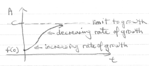
Key Features:

• Initial rapid (exponential-like) growth

• Growth rate decreases as population approaches

• Horizontal asymptote at

Example: Modeling the Spread of the Flu

The function models the number of people ill with influenza weeks after an outbreak in a town of 30,000.

• At (start): people

• At weeks: people

• Limiting value as : (entire population)

Newton’s Law of Cooling

Exponential Cooling Model

Newton’s Law of Cooling describes the temperature of an object as it cools in a surrounding medium of constant temperature :

• Formula:

  • = initial temperature of the object

  • = temperature of the surroundings

  • = negative constant (for cooling)

Example: An object heated to C is placed in a C room. After 5 minutes, its temperature is C.

• Given: , , at

• Solving for :

• Model:

• After 20 minutes: C

• To find when C:

  • minutes

Expressing Any Exponential Equation in Base e

Conversion to Base e

Any exponential equation of the form can be rewritten in terms of base :

• Since , then

• So,

Example 1: Rewrite in base :

Example 2: Rewrite in base :

• This matches the exponential growth model with (or 1.7% growth rate).