Randomness and Probability

Random Phenomena and Empirical Probability

Random phenomena are processes where individual outcomes cannot be predicted, but the long-run behavior can be understood. Each attempt (trial) produces an outcome, and outcomes can be grouped into events. The sample space is the set of all possible outcomes, denoted as S or Ω. Empirical probability is the long-run relative frequency of an event, based on repeated observation. The Law of Large Numbers (LLN) states that as the number of trials increases, the relative frequency of an event approaches a single value, provided the events are independent.

• Trial: Each attempt in a random process.

• Outcome: The result of a trial.

• Event: A set of outcomes or a combination of outcomes.

• Sample Space: The collection of all possible outcomes.

• Empirical Probability: Probability based on observed data.

• Independence: One trial's outcome does not affect another.

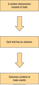
Example: Tossing a coin repeatedly: Each toss is a trial, the outcome is heads or tails, and the event could be getting heads.

The Nonexistent Law of Averages

Many confuse the Law of Large Numbers with the so-called "Law of Averages," which incorrectly suggests that things must even out in the short run. The Law of Averages does not exist; only long-run behavior is predictable.

Types of Probability

Probability can be estimated in three ways:

• Empirical Probability: Based on observed data.

• Theoretical Probability: Calculated when outcomes are equally likely, using the formula:

$ P(A) = \frac{\text{Number of outcomes in } A}{\text{Number of possible outcomes}} $

• Subjective Probability: Based on personal judgment or experience, not on data or equally likely outcomes. Subjective probability is prone to biases such as overconfidence, sunk cost, and recency bias.

Probability Rules

Probability rules help combine and calculate probabilities for events:

• Rule 1: Probability is between 0 and 1. $ 0 \leq P(A) \leq 1 $

• Rule 2 (Assignment Rule): The probability of the sample space is 1. $ P(S) = 1 $

• Rule 3 (Complement Rule): $ P(A^C) = 1 - P(A) $ where $A^C$ is the complement of A.

• Rule 4 (Multiplication Rule for Independent Events): $ P(A \text{ and } B) = P(A) \times P(B) $ if A and B are independent.

• Rule 5 (Addition Rule for Disjoint Events): $ P(A \text{ or } B) = P(A) + P(B) $ if A and B are disjoint.

• Rule 6 (General Addition Rule): $ P(A \text{ or } B) = P(A) + P(B) - P(A \text{ and } B) $

Joint Probability and Contingency Tables

Contingency tables organize data for two categorical variables, showing joint, marginal, and conditional probabilities. Marginal probabilities are found in the table's margins, joint probabilities in the interior, and conditional probabilities are calculated given one event.

• Marginal Probability: $ P( ext{woman}) = \frac{251}{478} = 0.525 $

• Joint Probability: $ P( ext{woman and camera}) = \frac{91}{478} = 0.190 $

• Conditional Probability: $ P( ext{bike} | ext{woman}) = \frac{30}{251} = 0.120 $

Conditional Probability and Independence

Conditional probability is the probability of event B given event A, written as $ P(B|A) $. The general multiplication rule calculates the probability of both events occurring, regardless of independence:

$ P(A \text{ and } B) = P(A) \times P(B|A) $

Events A and B are independent if $ P(B|A) = P(B) $. Disjoint events cannot be independent.

Constructing Contingency Tables

Given probabilities, you can construct a contingency table to find other probabilities. Marginal probabilities go in the margins, joint probabilities in the interior. Probabilities in the cells add up to the marginal totals.

Probability Trees

Probability trees visually represent the probabilities of multiple events, including conditional probabilities. Each branch shows the probability of an event, and joint probabilities are calculated by multiplying along the branches. All joint events in a tree are disjoint, so their probabilities can be added.

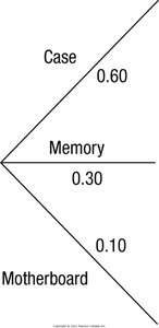
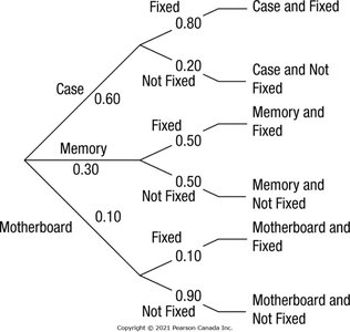
Example: In a manufacturing process, the probability that a minor adjustment will correct a problem is calculated by summing the joint probabilities of each adjustment and outcome.

$ P( ext{Fixed}) = P( ext{Case and Fixed}) + P( ext{Memory and Fixed}) + P( ext{Motherboard and Fixed}) $

For the given example, the likelihood that a minor adjustment will correct the problem is about 64%.

Bayes’s Rule

Bayes’s Rule allows us to reverse conditioning and update probability estimates given new information. For mutually exclusive and exhaustive events $A_i$:

$ P(A_i|B) = \frac{P(B|A_i) \times P(A_i)}{\sum_{j=1}^n P(B|A_j) \times P(A_j)} $

Bayes’s Rule is essential for updating probabilities when additional information is available.

Common Pitfalls in Probability

• Probabilities must add up to 1.

• Only add probabilities for disjoint events.

• Only multiply probabilities for independent events.

• Do not confuse disjoint and independent events.

Summary of Key Concepts

• Probability is based on long-run relative frequencies.

• The Law of Large Numbers describes long-run behavior, not short-run balancing.

• Probability can be estimated empirically, theoretically, or subjectively.

• Basic rules help combine probabilities for complex events.

• Independence and disjointness are distinct concepts.

• Probability trees and Bayes’s Rule are tools for updating and representing probabilities.