Chapter 4: Describing the Relation Between Two Variables

4.1 Scatter Diagrams and Correlation

Scatter Diagrams

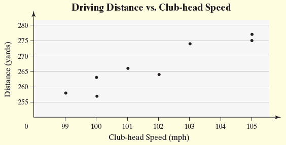
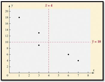
Scatter diagrams are graphical tools used to visualize the relationship between two quantitative variables measured on the same individuals. The explanatory variable is plotted on the horizontal (x-axis), and the response variable is plotted on the vertical (y-axis). Each point represents an individual observation.

• Explanatory Variable (X): The variable that explains or predicts changes in the response variable.

• Response Variable (Y): The variable whose value is explained by the explanatory variable.

• Scatter Diagram: Used to identify patterns such as linear, nonlinear, or no relation between variables.

• Interpretation: Patterns in the scatter diagram help determine the type and strength of the relationship.

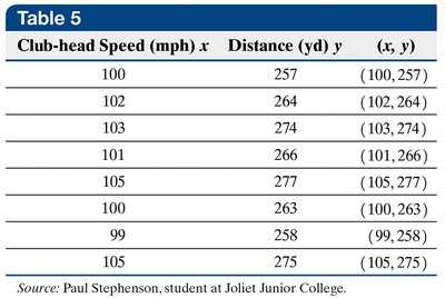
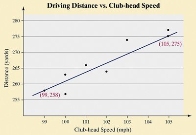
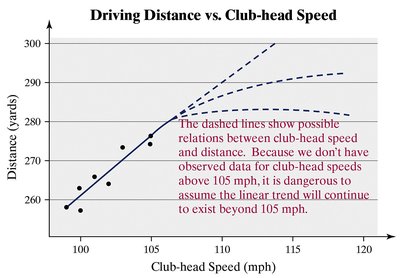
• Example: Club-head speed (mph) vs. driving distance (yards) in golf.

Association Types

• Positive Association: As one variable increases, the other also increases.

• Negative Association: As one variable increases, the other decreases.

• No Association: No discernible pattern between variables.

Linear Correlation Coefficient (Pearson's r)

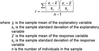
The linear correlation coefficient (r) measures the strength and direction of the linear relationship between two quantitative variables. The population correlation coefficient is denoted by , and the sample correlation coefficient by r.

• Formula:

• Properties:

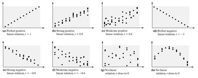
  • r ranges from -1 to 1.

  • r = +1: Perfect positive linear relation.

  • r = -1: Perfect negative linear relation.

  • r close to 0: Little or no linear relation.

  • r is unitless.

  • r is not resistant to outliers.

Computing and Interpreting r

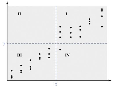
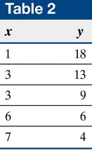
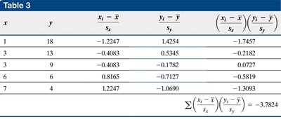
• Calculate means and standard deviations for x and y.

• Standardize values and multiply corresponding pairs.

• Sum the products and divide by n-1.

• Interpret the value of r based on its sign and magnitude.

Testing for a Linear Relation

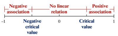
• Determine the absolute value of r.

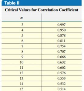
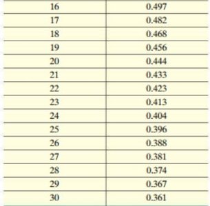
• Compare to the critical value from a table based on sample size.

• If |r| > critical value, a linear relation exists.

Correlation vs. Causation

• Correlation: Indicates association, not causation.

• Causation: Requires evidence that changes in one variable directly cause changes in another.

• Lurking Variable: A third variable that affects both explanatory and response variables, potentially confounding results.

• Example: Air temperature affects both air-conditioning bills and crime rates, but does not imply causation between the two.

4.2 Least-Squares Regression

Least-Squares Regression Line

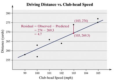
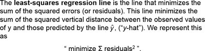
The least-squares regression line is the line that minimizes the sum of squared residuals (errors) between observed and predicted values of the response variable. It is used to make predictions and describe linear relationships.

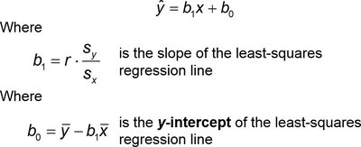
• Equation:

• Slope:

• Y-intercept:

Interpretation of Slope and Y-Intercept

• Slope: Represents the average change in the response variable for a one-unit increase in the explanatory variable.

• Y-intercept: Represents the predicted value of the response variable when the explanatory variable is zero. Only interpret if zero is a reasonable value and observed in the data.

• Scope of Model: Predictions should not be made for values outside the observed range of the explanatory variable.

4.4 Contingency Tables and Association

Contingency Tables

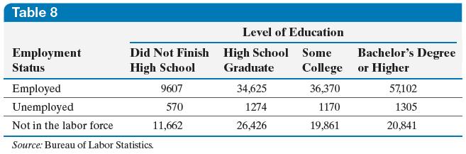
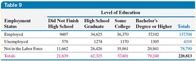
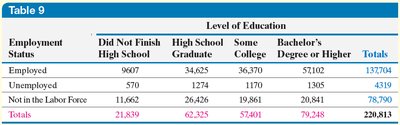
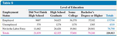
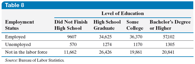
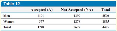
A contingency table (or two-way table) displays the frequency distribution of two categorical variables. Rows represent one variable, columns represent another, and each cell shows the count for a specific combination.

Marginal Distribution

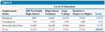
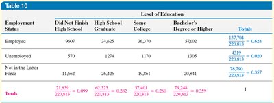
• Marginal Distribution: The frequency or relative frequency distribution of either the row or column variable, summing across the other variable.

• Example: Marginal distribution of employment status or education level.

Conditional Distribution and Association

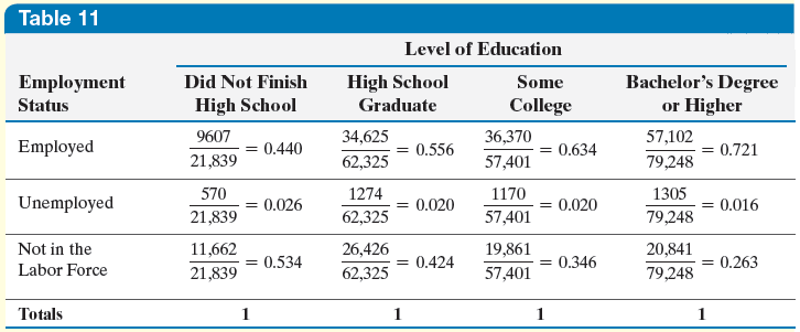
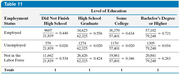
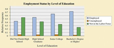
• Conditional Distribution: The relative frequency of each category of the response variable, given a specific value of the explanatory variable.

• Association: If conditional distributions differ across categories of the explanatory variable, an association exists.

• Example: Proportion employed by education level.

Simpson's Paradox

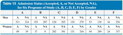
• Simpson's Paradox: An association between two variables reverses or disappears when a third variable is introduced.

• Example: Gender bias in university admissions appears in aggregate data, but disappears when program of study is considered.

Summary Table: Types of Relationships in Scatter Diagrams

Additional info: Academic context and examples were expanded for clarity and completeness. Tables were recreated and summarized for study purposes.