Exploring Data with Tables and Graphs

Frequency Distributions for Organizing and Summarizing Data

Frequency distributions are fundamental tools in statistics for organizing and summarizing large sets of quantitative data. They display how often each value or range of values occurs in a dataset, making it easier to identify patterns and trends.

• Definition: A frequency distribution is a table that lists classes (intervals) of data values along with their corresponding frequencies.

• Purpose: To provide a clear summary of the data, facilitating further analysis and visualization.

• Example: A frequency distribution of commute times might show how many people fall into each time interval.

Histograms

A histogram is a graphical representation of a frequency distribution. It consists of adjacent bars, where each bar represents a class interval and its height corresponds to the frequency of data within that interval.

• Definition: A histogram is a bar graph with equal-width bars drawn adjacent to each other, representing the frequency of quantitative data values.

• Horizontal Scale: Represents classes of quantitative data values.

• Vertical Scale: Represents frequencies.

• Key Uses:

  • Displays the shape of the data distribution

  • Shows the location of the center

  • Shows the spread of the data

  • Identifies outliers

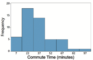
• Example: The histogram below shows the frequency of commute times in minutes.

Relative Frequency Histograms

Relative frequency histograms are similar to standard histograms, but the vertical axis represents the proportion (relative frequency) of data in each class, rather than the absolute frequency.

• Definition: A relative frequency histogram displays the same shape and horizontal scale as a histogram, but the vertical scale shows relative frequencies (percentages).

• Purpose: Useful for comparing distributions with different sample sizes.

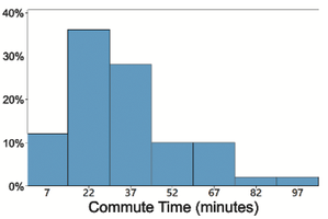
• Example: The relative frequency histogram below shows the percentage of people in each commute time interval.

Critical Thinking: Interpreting Histograms

Histograms allow for critical analysis of data using the CVDOT framework:

• Center: Where most data values are concentrated.

• Variation: The spread or dispersion of the data.

• Distribution: The overall shape of the data (e.g., symmetric, skewed).

• Outliers: Data points that are significantly different from others.

• Time: If applicable, how data changes over time.

Common Distribution Shapes

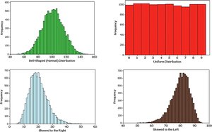
Understanding the shape of a distribution is essential for interpreting data. Common shapes include normal (bell-shaped), uniform, skewed right, and skewed left distributions.

• Normal Distribution: Symmetric, bell-shaped curve.

• Uniform Distribution: All values have approximately the same frequency.

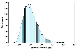
• Skewed Right: Longer tail on the right side.

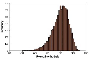
• Skewed Left: Longer tail on the left side.

• Example: The image below illustrates these common distribution shapes.

Normal Distribution

A normal distribution is characterized by its symmetric, bell-shaped curve. Many natural phenomena follow this distribution, making it a cornerstone of statistical analysis.

• Definition: A distribution where data is symmetrically distributed around the mean, forming a bell-shaped curve.

• Properties:

  • Mean, median, and mode are equal

  • 68% of data falls within one standard deviation of the mean

  • 95% within two standard deviations

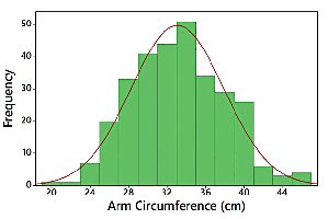
• Example: The histogram below shows arm circumference data with a normal distribution.

Skewness

Skewness describes the asymmetry of a distribution. If a distribution is not symmetric, it is said to be skewed.

• Definition: Skewness is a measure of the degree to which a distribution is not symmetric.

• Right (Positive) Skew: The tail extends more to the right.

• Left (Negative) Skew: The tail extends more to the left.

Assessing Normality with Normal Quantile Plots

Normal quantile plots (also called Q-Q plots) are used to assess whether a dataset follows a normal distribution. The pattern of points in the plot is compared to a straight line.

• Criteria for Normality:

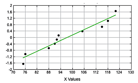
  • If the points are reasonably close to a straight line and do not show a systematic pattern, the distribution is normal.

  • If the points deviate from a straight line or show a systematic pattern, the distribution is not normal.

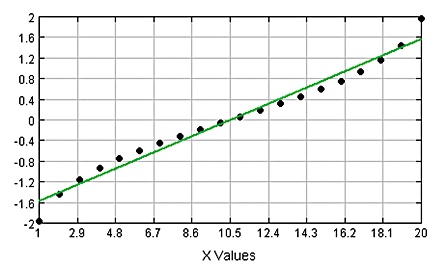
• Example: The following images illustrate normal and non-normal distributions using normal quantile plots.

  • Normal Distribution:

  • Not a Normal Distribution (points not close to straight line):

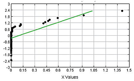
  • Not a Normal Distribution (systematic pattern):

Summary Table: Distribution Shapes and Their Properties

The table below summarizes the main types of distribution shapes and their key properties.

Key Formulas

• Relative Frequency:

• Skewness Coefficient: where is sample size, is each data value, is the mean, and is the standard deviation.