Chapter 1: Introduction to Statistics and Collecting Data

Types of Variables

Variables are characteristics or attributes that can take on different values. Understanding the types of variables is fundamental in statistics.

• Qualitative (Categorical) Variables: Classify individuals based on attributes or characteristics (e.g., gender, color).

• Quantitative Variables: Provide numerical measures. Values can be meaningfully added or subtracted.

  • Discrete Variable: Has a finite or countable number of possible values (e.g., number of students).

  • Continuous Variable: Has an infinite number of possible values, measurable to any desired accuracy (e.g., height, time).

Parameter: Numerical summary of a population. Statistic: Numerical summary based on a sample.

Levels of Measurement

• Nominal: Names, labels, or categorizes; no ranked order.

• Ordinal: Properties of nominal, but values can be ranked.

Sampling Methods

Sampling is the process of selecting a subset of individuals from a population to estimate characteristics of the whole population.

• Simple Random Sample: Each individual has an equal chance of being selected.

• Stratified Sample: Population divided into strata; random sample from each stratum.

• Systematic Sample: Select every k-th individual after a random start.

• Cluster Sample: Population divided into groups; select entire groups randomly.

• Convenience Sample: Individuals easily obtained; may not be representative.

Types of Studies

• Observational Study: Researcher observes without intervention.

• Case-Controlled Study: Sample divided into groups based on behavior.

• Experimental Study: Researcher manipulates variables to observe effects.

• Confounding Variables: Variables that affect each other, making it hard to distinguish their effects.

• Treatment Group: Receives the treatment.

• Control Group: Does not receive the treatment.

Chapter 2: Describing Data with Tables and Graphs

Relative Frequency and Distributions

Relative frequency is the proportion of observations within a category.

• Relative Frequency Formula:

• Relative Frequency Distribution: Lists each category with its relative frequency; proportions sum to 1.

Graphical Representations

• Bar Graph: Categories on one axis, frequency/relative frequency on the other; rectangles represent frequencies.

• Pareto Chart: Bar graph with bars in decreasing order of frequency.

• Side-by-Side Graphs: Compare data using relative frequencies.

• Pie Chart: Circle divided into sectors proportional to category frequency.

• Histogram: Rectangles for each class; rectangles touch, representing frequency or relative frequency.

Chapter 3: Describing Data Numerically

Measures of Central Tendency

Central tendency describes the center of a data set.

• Mean: Average value.

• Median: Middle value when data is ordered.

• Mode: Most frequently occurring value.

Skewness

• Left Skewed: Mean < Median

• Symmetric: Mean = Median

• Right Skewed: Mean > Median

Measures of Spread

• Range:

• Variance: Measures average squared deviation from the mean.

• Standard Deviation: Square root of variance; measures spread.

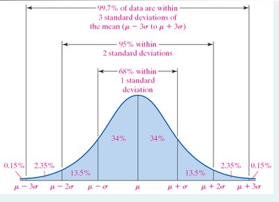
Empirical Rule

If the distribution is bell-shaped:

• 68% of data within 1 standard deviation of the mean

• 95% within 2 standard deviations

• 99.7% within 3 standard deviations

Z-Score

The z-score measures the distance of a data value from the mean in units of standard deviation.

• Z-Score Formula:

• Z-score is unitless; mean = 0, standard deviation = 1.

• Extreme outlier: z < -3.0 or z > 3.0

Percentiles and Quartiles

• Percentile Formula: , where i is the term number for the k-th percentile.

• Quartiles:

  • Q1:

  • Q2:

  • Q3:

• Interquartile Range (IQR):

• Lower Fence:

• Upper Fence:

Five-Number Summary

• Minimum

• First Quartile (Q1)

• Median (Q2)

• Third Quartile (Q3)

• Maximum

Chapter 5: Probability

Probability Concepts

Probability quantifies the likelihood of an event occurring.

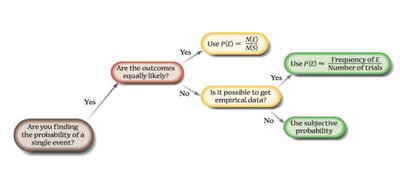
• Theoretical Probability: All outcomes equally likely.

• Empirical Probability: Based on observed data.

Disjoint (Mutually Exclusive) Events

• Events with no outcomes in common.

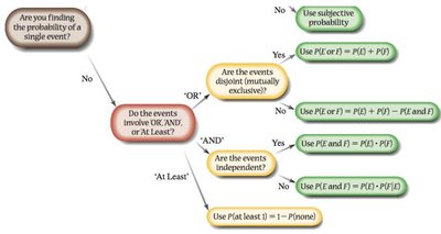
• Addition Rule for Disjoint Events:

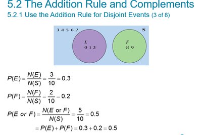
General Addition Rule

• For any two events:

Complement Rule

• The complement of event E is all outcomes not in E.

Independent and Dependent Events

• Independent: Occurrence of one event does not affect the other.

• Dependent: Occurrence of one event affects the probability of the other.

• Multiplication Rule for Independent Events:

• Multiplication Rule for n Independent Events:

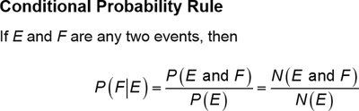
Conditional Probability

Conditional probability is the probability of event F given that event E has occurred.

• Conditional Probability Formula:

Multiplication Rule of Counting

• If a task consists of a sequence of choices, multiply the number of options for each step.

• Example: If there are 3 choices for the first step and 2 for the second, total ways = 3 × 2 = 6.

Permutations and Combinations

• Permutation: Ordered arrangement; no repetition.

• Combination: Unordered selection; no repetition.

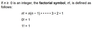
• Factorial: ; ,

Probability Rules Flowcharts

Chapter 6: Binomial Distribution & Discrete Random Variables

Random Variables

A random variable represents possible numerical values from a random event.

• Discrete Random Variable: Can assume only a countable number of values (e.g., number of complaints per day).

• Continuous Random Variable: Can assume any value on a continuum (e.g., time, height).

Discrete Probability Distribution

• List of all possible pairs [xi, P(xi)]

• xi: Value of random variable

• P(xi): Probability associated with xi

• xi’s are mutually exclusive and collectively exhaustive

• 0 ≤ P(xi) ≤ 1 for each xi

• Sum of all probabilities = 1

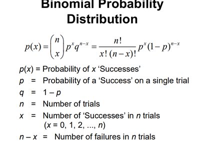
Binomial Distribution

The binomial distribution models the number of successes in a fixed number of independent trials, each with the same probability of success.

• n: Number of trials

• p: Probability of success

• q: Probability of failure (q = 1 - p)

• x: Number of successes in n trials

• Trials are independent

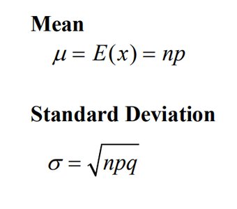
Mean and Standard Deviation of Binomial Distribution

• Mean:

• Standard Deviation:

Chapter 7: Continuous Probability Distributions

Uniform Distribution

A uniform distribution is a type of continuous probability distribution where all outcomes are equally likely within a certain interval.

• Probability is constant across the interval.

• Used to model situations where each outcome in a range is equally likely.