Descriptive vs. Inferential Statistics

Definitions and Applications

Descriptive statistics summarize and describe the features of a dataset, while inferential statistics use sample data to make generalizations about a population.

• Descriptive statistics: Include measures such as averages, percentages, tables, graphs, and ranges. They describe the data you have collected.

• Inferential statistics: Allow you to infer or predict characteristics of a larger population based on a sample.

• Example: Surveying 100 students and calculating their average study hours is descriptive; using that average to estimate the study hours for all students is inferential.

Samples, Populations, Statistics, and Parameters

Key Terms and Relationships

Understanding the distinction between samples and populations is fundamental in statistics.

• Population: The entire group you want to study.

• Sample: A subset of the population selected for analysis.

• Parameter: A numerical value that describes a characteristic of the population.

• Statistic: A numerical value that describes a characteristic of the sample.

• Example: The average age of all students (parameter) vs. the average age of a sample of 100 students (statistic).

Representative Samples

Importance in Statistical Inference

A representative sample accurately reflects the characteristics of the population, ensuring valid inferences.

• Key Point: Sampling bias can lead to incorrect conclusions about the population.

Sampling Procedures

Types of Sampling Methods

Different sampling methods are used to select samples from populations.

• Random Sampling: Every member has an equal chance of being selected.

• Stratified Sampling: Population divided into groups (strata), and samples are taken from each group.

• Cluster Sampling: Population divided into clusters, and entire clusters are randomly selected.

• Convenience Sampling: Samples are taken from individuals who are easiest to reach.

• Example Table:

Observational vs. Experimental Research

Research Designs and Causality

• Observational: Researchers observe without intervention; cannot establish causality.

• Experimental: Researchers manipulate variables; can provide evidence for cause and effect.

• Example: Observing exercise habits vs. assigning exercise routines.

Quantitative Variables: Discrete vs. Continuous

Classification of Variables

• Discrete: Countable values (e.g., number of children).

• Continuous: Measurable values within a range (e.g., height, weight).

• Example: Number of siblings is discrete; height is continuous.

Scales of Measurement

Types of Measurement Scales

• Nominal: Categories without order (e.g., eye color).

• Ordinal: Ordered categories (e.g., satisfaction level).

• Interval: Ordered, meaningful differences, no true zero (e.g., temperature).

• Ratio: Ordered, meaningful differences, true zero (e.g., weight).

Random Error vs. Systematic Error

Types of Measurement Error

• Random Error: Unpredictable variation; can be reduced by averaging.

• Systematic Error: Consistent bias; must be corrected at the source.

• Example: Fluctuating scale readings (random) vs. consistently miscalibrated scale (systematic).

Visual Displays of Data

Interpreting Common Graphs

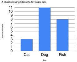
• Bar Graph: Compares categories; tallest bar shows highest frequency.

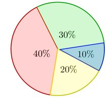
• Pie Chart: Shows parts of a whole; largest slice represents largest percentage.

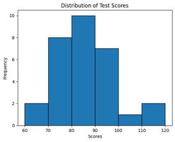
• Histogram: Shows distribution of numerical data; bars touch, representing intervals.

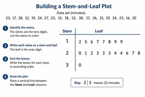
• Stem-and-Leaf Plot: Displays numerical data by place value; keeps original values visible.

Measures of Central Tendency: Mean, Median, Mode

Calculating and Interpreting

• Mean: Average; sum of values divided by number of values.

• Median: Middle value when data are ordered.

• Mode: Most frequently occurring value.

• Example: For 4, 6, 6, 8, 11: Mean = 7, Median = 6, Mode = 6.

Effect of Outliers

Impact on Mean, Median, and Mode

• Mean: Strongly affected by outliers.

• Median: Resistant to outliers.

• Mode: Usually unaffected unless the outlier is frequent.

• Example: Adding 100 to 10, 11, 12, 13, 14 shifts the mean but not the median or mode.

Boxplots (Box-and-Whisker Plots)

Interpreting Boxplots

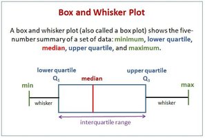
Boxplots display the five-number summary: minimum, first quartile (Q1), median, third quartile (Q3), and maximum.

• Minimum: Smallest value

• Q1: 25% below this value

• Median: Middle value

• Q3: 75% below this value

• Maximum: Largest value

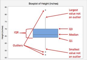
• Interquartile Range (IQR):

• Outliers: Values outside the whiskers may be marked as outliers.

Variance and Standard Deviation

Measuring Spread

Variance and standard deviation quantify how much data values deviate from the mean.

• Variance: Average of squared differences from the mean.

• Standard Deviation: Square root of variance.

• Population vs. Sample: Population variance divides by N; sample variance divides by n-1.

• Example: For 2, 4, 6: Mean = 4, Variance = 2.67, Standard deviation ≈ 1.63.

Percentiles and Z-Scores

Calculating Percentiles

To determine the percentile of a score, calculate its z-score and use the normal distribution.

• Z-score formula:

• Percentile: Use z-score to find the percentage of scores below the given value.

• Example: Score = 85, Mean = 75, SD = 10: , percentile ≈ 84th.

Central Limit Theorem

Sampling Distributions

The Central Limit Theorem states that the distribution of sample means approaches normality as sample size increases, regardless of population distribution.

• Mean of sampling distribution:

• Standard error:

• Example: Population mean = 100, SD = 20, n = 25: Standard error = 4.

Additional info: All explanations are expanded for clarity and completeness, suitable for exam preparation in an introductory statistics course.