Numerical Summaries of Data: Measures of Center, Dispersion, and Position

스터디 가이드 - 스마트 노트

자료에 맞춘 맞춤형 노트, 핵심 정의, 예시, 맥락을 확장해 제공합니다.

Numerical Summaries of Data

Descriptive Statistics with Technology

Descriptive statistics summarize and describe the main features of a dataset. Calculators and statistical software can quickly compute these summaries, which include measures of center, dispersion, and position.

TI-84 Calculator: Use the '1-Var Stats' function to compute most descriptive statistics except variance and interquartile range (IQR).
Minitab: Use the 'Display Descriptive Statistics' option under 'Basic Statistics' to compute a variety of statistics for selected variables.

Measures of Center

Mean

The mean is the arithmetic average of a dataset, calculated as the sum of all observations divided by the number of observations. It is a common measure of the center of quantitative data.

Population mean ($\mu$):
Sample mean ($\bar{x}$):
The mean is sensitive to extreme values (outliers).

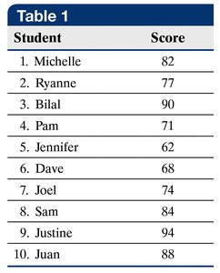
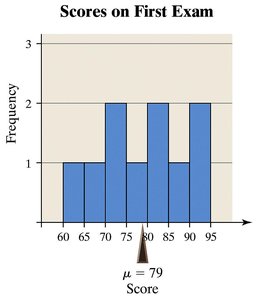
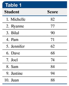
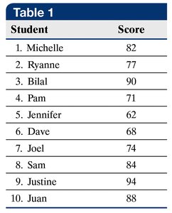
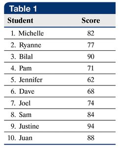
Example: The following table shows the scores of 10 students. The population mean is $\mu = 79$.

Table of student scores

Mean as a Measure of Center

The mean can be interpreted as the dataset's center of gravity. In a histogram, the mean is the balance point.

Histogram showing mean as balance point

Median

The median is the value that lies in the middle of the dataset when the observations are arranged in ascending order. It divides the data into two equal halves.

Denoted as $M$.
Resistant to outliers.

Example: For the same dataset, the median is $M = 79.5$.

Comparing Mean and Median

When a dataset contains outliers or is skewed, the mean and median can differ significantly. The median is a better measure of center for skewed data or data with outliers.

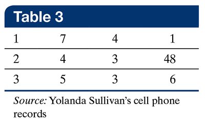
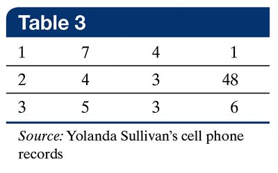
Comparison of mean and median in skewed and symmetric distributions

Example: Yolanda's phone call lengths have a mean of 7.25 and a median of 3.5. The mean is influenced by one long call (48 minutes), making the median a better descriptor of a typical call.

Table of phone call lengths

Mode

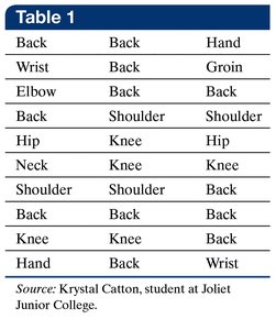
The mode is the most frequently occurring value in a dataset. A dataset can have one mode, more than one mode, or no mode at all. The mode is useful for both quantitative and qualitative data.

Example: In the following table, the mode is "Back" because it appears most frequently.

Table of body part injuries

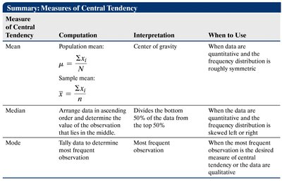
Summary Table: Measures of Central Tendency

Measure of Central Tendency	Computation	Interpretation	When to Use
Mean	Population: Sample:	Center of gravity	Quantitative data, roughly symmetric distribution
Median	Middle value in ordered data	Divides bottom 50% from top 50%	Quantitative data, skewed or with outliers
Mode	Most frequent observation	Most frequent observation	Qualitative data or when mode best describes center

Summary table of measures of central tendency

Measures of Dispersion

Dispersion

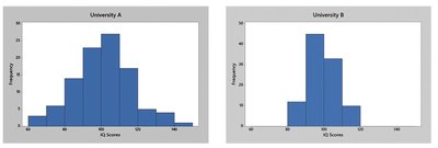
Dispersion refers to how spread out the values are from the center. Common measures include range, variance, standard deviation, and interquartile range (IQR).

Histograms showing different dispersions with same mean

Range

The range is the difference between the maximum and minimum values in a dataset.

Formula:

Example: For the student scores, .

Table of student scores for range calculation

Standard Deviation and Variance

The standard deviation (SD) measures the average distance of data points from the mean. The variance is the square of the standard deviation.

Population SD ($\sigma$):
Sample SD ($s$):
Population variance:
Sample variance:

Example: For the sample of Ryanne, Jennifer, Dave, and Juan, and .

Table of student scores for standard deviation calculation Table of student scores for variance calculation

Interquartile Range (IQR)

The interquartile range (IQR) measures the spread of the middle 50% of the data and is resistant to outliers.

Formula:
Q1: First quartile (25th percentile)
Q3: Third quartile (75th percentile)

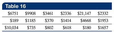
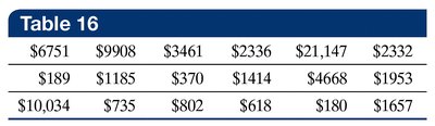
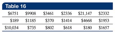
Example: For the collision coverage claims data, , , so .

Table of collision coverage claims

Summary Table: Measures of Dispersion

Range: Measures total variation.
Standard deviation: Measures average variation from the mean.
Variance: Square of the standard deviation.
IQR: Measures variation of the middle half; resistant to outliers.
Measures of dispersion cannot be negative.

Measures of Position

z-Score

The z-score indicates how many standard deviations a value is from the mean. It is used to compare values from different datasets or to identify unusual values.

Formula:
z-scores farther from 0 indicate more unusual values.
z-scores ≥ 2 or ≤ -2 are generally considered abnormal.

Example: A score of 73 on two exams with different means and standard deviations yields different z-scores, indicating relative performance.

Empirical Rule

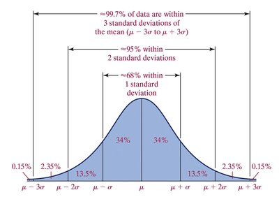
The Empirical Rule applies to bell-shaped (normal) distributions:

About 68% of data within 1 SD of the mean
About 95% within 2 SDs
About 99.7% within 3 SDs

Empirical Rule illustration on normal curve

Chebyshev’s Inequality

Chebyshev’s Inequality applies to any dataset, regardless of shape. At least of the data lies within standard deviations of the mean, for .

For , at least 75% of data is within 2 SDs of the mean.

Percentiles and Quartiles

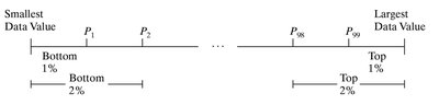
Percentiles indicate the relative standing of a value within a dataset. The th percentile () is the value below which $k$ percent of the data falls.

Median is the 50th percentile ().
First quartile () is the 25th percentile ().
Third quartile () is the 75th percentile ().

Percentile diagram Quartile diagram

Identifying Outliers

Upper and Lower Fences

Outliers can be identified using the IQR and quartiles:

Lower fence:
Upper fence:
Values outside these fences are considered outliers.

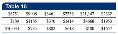
Example: For the collision claims data, the only outlier is $21,147, which exceeds the upper fence.

Table of collision coverage claims for outlier identification

Five-Number Summary and Boxplot

Five-Number Summary

The five-number summary consists of the minimum, first quartile (), median, third quartile (), and maximum. It provides a concise summary of the distribution of a dataset.

Can be visualized using a boxplot.
Boxplots display the spread and identify outliers.

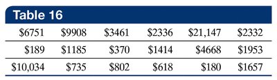
Example: For the collision claims data, the five-number summary is:

Minimum: $189
Q1: $735
Median: $1,805
Q3: $4,668
Maximum: $21,147

Table of collision coverage claims for five-number summary Boxplot for collision coverage claims

Boxplots in Software

Minitab: Can create simple and side-by-side boxplots for visual comparison of distributions.