Chapter 3: Numerically Summarizing Data

3.1 Measures of Central Tendency

Measures of central tendency are statistical values that describe the center of a data set. The most common measures are the mean, median, and mode. These measures help summarize and interpret data efficiently.

3.1.1 Arithmetic Mean

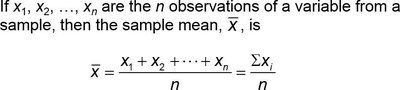
The arithmetic mean is the sum of all values divided by the number of observations. It is used for both populations and samples, but the notation differs:

• Population Mean (μ): Uses all individuals in the population and is a parameter.

• Sample Mean (\(\bar{x}\)): Uses a subset of the population and is a statistic.

Formula:

Example: The scores of 10 students in Table 1:

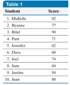
Population mean:

Sample mean (random sample of 4):

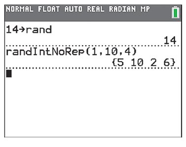
3.1.2 Median

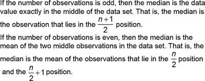
The median is the middle value when data are arranged in ascending order. It divides the data into two equal halves.

• If the number of observations is odd, the median is the value at position .

• If even, the median is the mean of the values at positions and .

Example (Odd n): Song lengths from the 1970s:

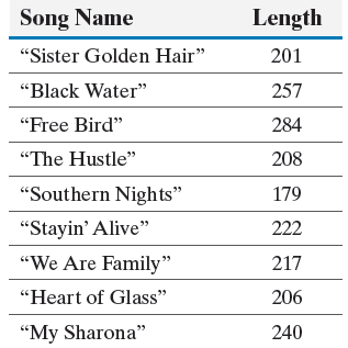
Median: 217 (5th value in ordered list)

Example (Even n): Test scores: 62, 68, 71, 74, 77, 82, 84, 88, 90, 94. Median:

3.1.3 Resistance of Statistics

A statistic is resistant if it is not substantially affected by extreme values. The median is resistant, while the mean is not.

Example: Cell phone call lengths:

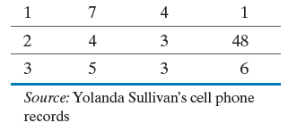
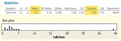
Mean = 7.25, Median = 3.50. The median better represents typical call length due to the outlier (48).

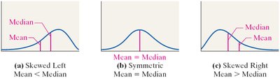
Relation to Distribution Shape:

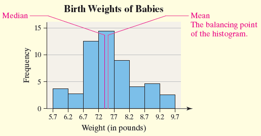
• Skewed left: Mean < Median

• Symmetric: Mean ≈ Median

• Skewed right: Mean > Median

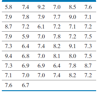
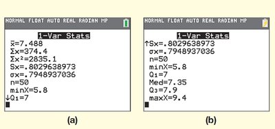
Example: Birth weights of babies (mean = 7.49, median = 7.35). Distribution is bell-shaped; mean and median are close.

3.1.4 Mode

The mode is the most frequent value in a data set. Data can have no mode, one mode, or multiple modes.

Example: O-ring failures: 0, 0, 0, ..., 1, 1, 1, 2, 3. Mode = 0 (occurs 17 times).

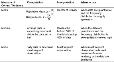
Summary Table: Measures of Central Tendency

3.2 Measures of Dispersion

Measures of dispersion describe the spread or variability of a data set. Common measures include range, standard deviation, and variance.

3.2.1 Range

The range is the difference between the largest and smallest values:

Example: Exam scores: Largest = 94, Smallest = 62, Range = 32.

3.2.2 Standard Deviation

The standard deviation measures the average distance of data values from the mean. It is calculated differently for populations and samples.

• Population Standard Deviation (σ):

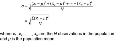
Computational formula:

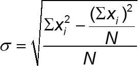
• Sample Standard Deviation (s):

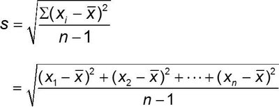
Computational formula:

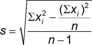
Example: Standard deviation for University A and B IQ scores:

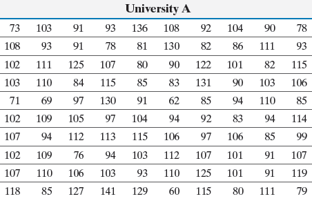
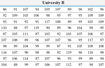
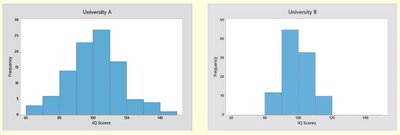
University A: s = 16.1, University B: s = 8.4. University A has more dispersion.

3.2.3 Variance

The variance is the square of the standard deviation:

• Population variance:

• Sample variance:

Example: If , then .

3.2.4 Empirical Rule (Bell-Shaped Distributions)

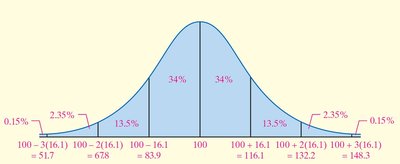
The Empirical Rule describes the spread of data in a normal (bell-shaped) distribution:

• 68% within 1 standard deviation ()

• 95% within 2 standard deviations ()

• 99.7% within 3 standard deviations ()

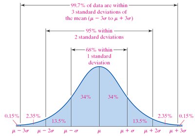
Example: University A IQ scores: Mean = 100, s = 16.1. 95% of scores between 67.8 and 132.2.

3.4 Measures of Position and Outliers

Measures of position describe the relative standing of a data value within a data set. Common measures include z-scores, percentiles, quartiles, and interquartile range.

3.4.1 z-Scores

A z-score indicates how many standard deviations a value is from the mean:

• Population:

• Sample:

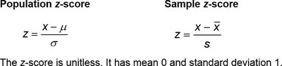
Example: Red Sox z-score:

3.4.2 Percentiles

The kth percentile () is the value below which k% of the data fall.

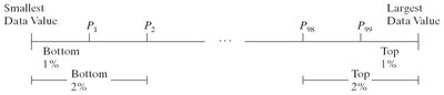
Example: SAT score of 600 in the 74th percentile means 74% scored ≤ 600.

3.4.3 Quartiles

Quartiles divide data into four equal parts:

• Q1: 25th percentile

• Q2: 50th percentile (median)

• Q3: 75th percentile

3.4.4 Interquartile Range (IQR)

The IQR is the range of the middle 50% of data:

Example: Q1 = $735, Q3 = $4668, IQR = $3933

3.4.5 Outliers

Outliers are values that fall outside the fences:

• Lower Fence:

• Upper Fence:

Values outside these fences are considered outliers.

3.5 The Five-Number Summary and Boxplots

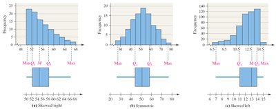
The five-number summary consists of: minimum, Q1, median, Q3, and maximum. Boxplots visually display these values and highlight outliers.

• Boxplots show the spread and symmetry of data.

• Whiskers extend to the smallest and largest values within the fences.

• Outliers are marked with asterisks.

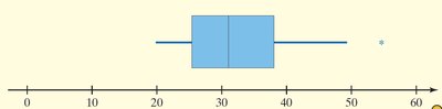
Example: Boxplots can be used to compare distribution shapes (skewed, symmetric).

Summary Table: Distribution Shape and Measures