Numerically Summarizing Data

Measures of Central Tendency

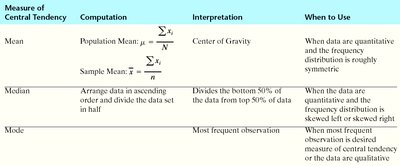
Measures of central tendency describe the center of a data set and are fundamental for understanding distributions. The three main measures are the mean, median, and mode.

• Mean: The arithmetic mean is the sum of all values divided by the number of observations. For a population, it is denoted by , and for a sample, by . Formula: Population mean: Sample mean: Interpretation: The mean represents the 'center of gravity' of the data. When to Use: When data are quantitative and the distribution is roughly symmetric.

• Median: The median is the middle value when data are ordered. If the number of observations is odd, it is the value at position . If even, it is the average of the two middle values. Interpretation: Divides the bottom 50% from the top 50% of data. When to Use: When the distribution is skewed left or right.

• Mode: The mode is the value that occurs most frequently. Interpretation: Most frequent observation. When to Use: When the most frequent observation is desired or for qualitative data.

Example: Music Video Counts

Consider the following data for music video counts:

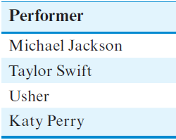
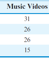
Mean: Median: Arrange values: 15, 26, 26, 31. Median = (26 + 26)/2 = 26. Mode: 26 (appears twice).

Relation Between Mean, Median, and Distribution Shape

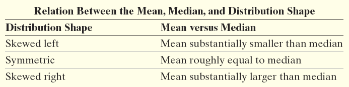
The relationship between the mean and median helps identify the shape of the distribution:

Measures of Dispersion

Measures of dispersion quantify the spread or variability of a data set. The main measures are range, variance, and standard deviation.

Range

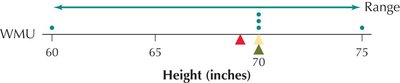
The range is the difference between the largest and smallest values in the data set.

• Formula: Range = Largest value – Smallest value

• Limitation: Sensitive to extreme values; ignores all values except extremes.

Standard Deviation and Variance

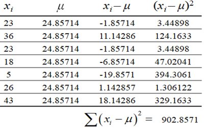
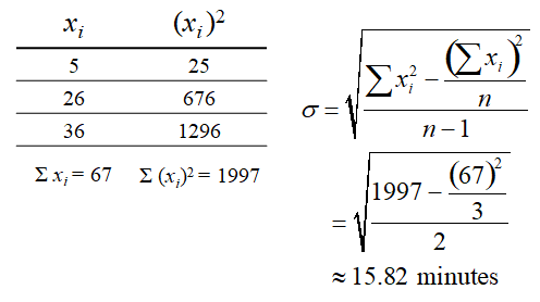
The standard deviation measures the average distance of data values from the mean. Variance is the square of the standard deviation.

• Sample Standard Deviation:

• Population Standard Deviation:

• Sample Variance:

• Population Variance:

Using Technology for Dispersion Measures

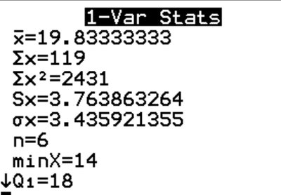
Statistical calculators can quickly compute mean, variance, and standard deviation for a data set.

Empirical Rule and Chebyshev's Rule

Empirical Rule

For bell-shaped (normal) distributions:

• About 68% of data falls within 1 standard deviation of the mean

• About 95% within 2 standard deviations

• About 99.7% within 3 standard deviations

Chebyshev's Rule

For any distribution, at least of data falls within standard deviations of the mean, where .

• For : At least 75% of data within 2 standard deviations

• For : At least 88.89% within 3 standard deviations

Measures of Position and Outliers

z-Scores

A z-score indicates how many standard deviations a value is from the mean.

• Sample z-score:

• Population z-score:

• Positive z-score: Value above mean; Negative: Below mean; Zero: Equal to mean.

Percentiles and Percentile Ranks

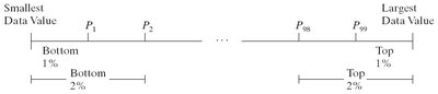
Percentiles indicate the relative position of a value in a data set.

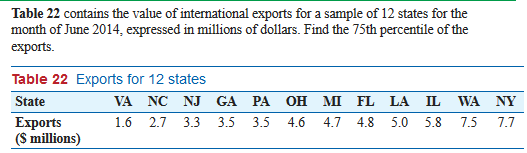
• The kth percentile, , is the value below which k% of data falls.

• Percentile rank of : Percentage of values less than or equal to $x$.

• To find the kth percentile: If is an integer, is the value at position $i$; otherwise, average the values at positions closest to $i$.

Quartiles

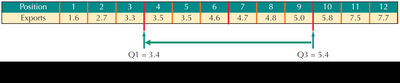
Quartiles divide the data into four equal parts:

• Q1: 25th percentile

• Q2: 50th percentile (median)

• Q3: 75th percentile

Interquartile Range (IQR)

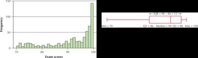
The IQR is a robust measure of spread, calculated as . It represents the spread of the middle 50% of the data.

Five-Number Summary and Boxplots

Five-Number Summary

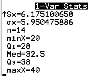
The five-number summary consists of:

• Minimum

• Q1

• Median (Q2)

• Q3

• Maximum

Boxplots

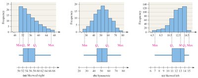
Boxplots graphically display the five-number summary and help visualize the distribution's shape and identify outliers.

• Box extends from Q1 to Q3, with a line at the median

• Whiskers extend to minimum and maximum values (excluding outliers)

• Outliers are marked separately

Distribution Shape and Boxplots

Boxplots can illustrate skewness:

• Skewed right: Longer whisker on the right, mean > median

• Symmetric: Whiskers and box are balanced, mean ≈ median

• Skewed left: Longer whisker on the left, mean < median

Detecting Outliers with IQR

A value is an outlier if it is:

• Below Q1 - 1.5(IQR)

• Above Q3 + 1.5(IQR)

Boxplots and quartiles are useful for describing the shape and identifying outliers in a distribution.