Scatterplots, Correlation, and Regression

Introduction

This section introduces the analysis of paired sample data using scatterplots, correlation, and regression. These tools are essential for understanding relationships between two quantitative variables and for making predictions based on observed data.

Scatterplots and Correlation

A scatterplot (or scatter diagram) is a graphical representation of paired quantitative data. The horizontal axis (x-axis) represents the first variable, and the vertical axis (y-axis) represents the second variable. Scatterplots are used to visually assess the relationship between two variables.

• Correlation: A correlation exists when the values of one variable are associated with the values of another variable.

• Linear Correlation: A linear correlation exists if the plotted points form a pattern that can be approximated by a straight line.

• No Correlation: If the plotted points do not show a distinct pattern, there is no correlation between the variables.

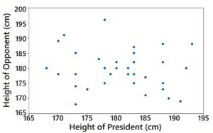
• Example: The scatterplot of heights of presidents and their main opponents shows no distinct pattern, indicating no correlation between the two variables.

Linear Correlation Coefficient (r)

The linear correlation coefficient, denoted by r, measures the strength and direction of the linear association between two variables. The value of r ranges from -1 to 1.

• r close to 1: Strong positive linear correlation.

• r close to -1: Strong negative linear correlation.

• r close to 0: No linear correlation.

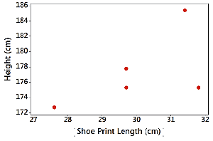
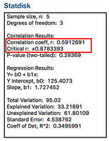
• Example: The correlation coefficient for shoe print length and height is r = 0.591, which is not clearly indicative of a strong linear correlation.

P-Value in Correlation Analysis

The P-value is the probability of obtaining a correlation coefficient as extreme as the observed value, assuming there is no linear correlation between the variables. It is used to assess the statistical significance of the observed correlation.

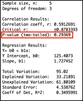
• High P-value (e.g., 0.294): Indicates a high chance of observing the correlation by random chance; insufficient evidence for linear correlation.

• Low P-value (e.g., 0.05 or less): Suggests the sample results are unlikely to occur by chance, supporting the existence of a linear correlation.

• Example: For shoe print length and height, a P-value of 0.294 means there is not sufficient evidence to conclude a linear correlation.

Scatterplot and Correlation: Larger Sample Example

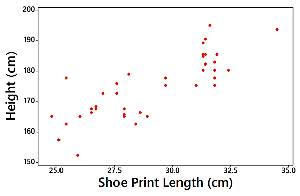
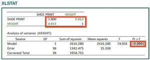
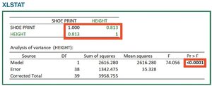
With a larger sample size (n = 40), the scatterplot of shoe print length and height shows a distinct pattern, and the correlation coefficient is r = 0.813 with a P-value < 0.0001. This provides strong evidence for a linear correlation between the two variables.

• Distinct pattern: Indicates a strong linear relationship.

• r = 0.813: Strong positive linear correlation.

• P-value < 0.0001: Very strong evidence against the null hypothesis of no correlation.

Regression Analysis

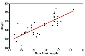
Regression is the process of finding the line (regression line or line of best fit) that best describes the relationship between two variables in paired sample data. The regression equation is used to make predictions about one variable based on the other.

• Regression Equation: The general form is where is the y-intercept and is the slope.

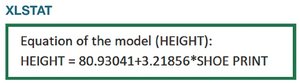
• Example: For shoe print length and height, the regression equation is Height = 80.9 + 3.22 × (Shoe Print Length).

• Interpretation: The slope indicates the change in height for each unit increase in shoe print length.

Summary Table: Correlation and Regression Results

The following table summarizes the key statistics for the correlation and regression analysis between shoe print length and height:

Additional info: The regression equation and correlation coefficient are calculated using statistical software and are interpreted in the context of the data. The slope and intercept values may vary depending on the sample size and data distribution.