Exponential Functions

Definition and Basic Properties

Exponential functions are a fundamental class of functions in calculus, widely used to model real-world phenomena such as population growth, radioactive decay, and compound interest. An exponential function is defined as follows:

• Definition: An exponential function is any function of the form , where and .

• Domain: All real numbers ().

• Range: All positive real numbers .

• Base: The constant is called the base of the exponential function.

Key Distinction: In , the variable is in the exponent, while in , the variable is the base. This distinction leads to very different behaviors and graphs.

Graphing Exponential Functions

Exponential functions can be graphed by plotting points for selected -values and connecting them with a smooth curve. The general shape depends on the base :

• If , the function increases as increases (exponential growth).

• If , the function decreases as increases (exponential decay).

• All graphs pass through the point since .

• The -axis () is a horizontal asymptote.

Theorems: Properties of Exponential Functions

• Theorem 1: The graph of is continuous, contains , and has the -axis as a horizontal asymptote.

• Theorem 2: For , , , and real , the following properties hold:

Exponential Functions with Base

The Natural Base

The number is an irrational constant approximately equal to . It is the base for natural exponential functions, which are especially important in calculus due to their unique properties in differentiation and integration.

• Definition: The natural exponential function is .

• Inverse: The inverse function is the natural logarithm, .

• Domain:

• Range:

Exponential Growth and Decay Models

Many real-world processes are modeled by exponential functions of the form , where is the initial amount and is the relative growth (or decay) rate.

• Exponential Growth: (e.g., population growth, bacteria growth)

• Exponential Decay: (e.g., radioactive decay, depreciation)

Example: Exponential Growth of Cholera Bacteria

The number of cholera bacteria grows according to , where is the initial number and is in hours.

• If , after hours: bacteria.

• After hours: bacteria.

Example: Exponential Decay of Carbon-14

Radioactive decay is modeled by , where is the initial amount and is in years.

• If mg, after years: mg.

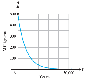
Half-Life and Graphical Solutions

The half-life of a substance is the time required for half of the initial amount to remain. For Carbon-14, the half-life can be estimated graphically or solved algebraically:

• Set and solve for in .

• Graphically, the intersection of and gives the half-life.

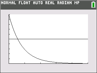
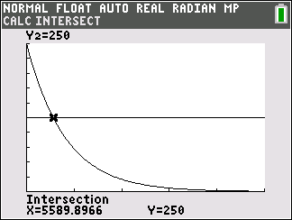
The calculated half-life is approximately years.

Exponential Regression and Data Modeling

Fitting Exponential Models to Data

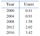
Exponential regression is used to fit an exponential model to observed data. This is common in business and economics for modeling growth trends.

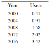
Scatterplot and Regression Analysis

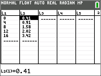
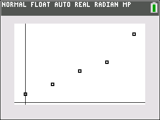
Data is entered into a calculator or software, and a scatterplot is created to visually assess the fit of an exponential model.

Finding the Regression Equation

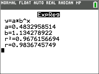
The regression equation is calculated, often yielding a model such as (rounded values). The value indicates the goodness of fit.

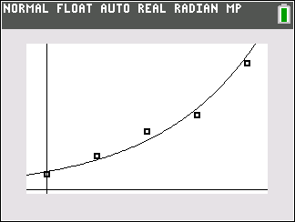
Prediction Example

To predict the number of internet users in 2024 ( years after 2000):

• billion users.

Applications: Compound Interest

Compound Interest Formula

Compound interest is interest calculated on both the initial principal and the accumulated interest from previous periods. The formula for compound interest is:

• Where is the future value, is the principal, is the annual interest rate (decimal), is the number of compounding periods per year, and is the number of years.

Example: deposited at annual rate, compounded monthly for $20$ years:

Continuous Compound Interest

When compounding occurs infinitely often, the formula becomes:

• Where

Example: invested at compounded continuously for $20$ years: