Financial Mathematics

Introduction to Financial Mathematics

Financial mathematics applies mathematical methods to solve problems related to finance, such as calculating interest, loan repayments, investments, and depreciation. Understanding these concepts is essential for making informed financial decisions.

Interest Calculations

Simple Interest

Simple interest is calculated only on the original principal amount throughout the investment or loan period. It is commonly used for short-term loans and some types of investments.

• Formula:

• Where:

  • = Final amount

  • = Principal (initial amount)

  • = Interest rate per period

  • = Number of periods

• Example: Investing R100 at 10% simple interest for 3 years yields R130.

Compound Interest

Compound interest is calculated on both the initial principal and the accumulated interest from previous periods. This leads to exponential growth over time and is widely used for savings and investments.

• Formula:

• Where: Same as above.

• Example: Investing R100 at 10% compound interest for 3 years yields R133.10.

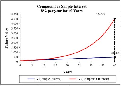
This graph illustrates how compound interest (red curve) grows much faster than simple interest (blue line) over 40 years at 8% per year.

Depreciation

Straight-Line (Simple) Depreciation

Depreciation is the reduction in the value of an asset over time. The straight-line method reduces the value by a fixed amount each year.

• Formula:

• Where:

  • = Value after years

  • = Initial value

  • = Depreciation rate per period

  • = Number of periods

Reducing-Balance (Compound) Depreciation

The reducing-balance method applies depreciation to the current value each period, resulting in a decreasing amount of depreciation each year.

• Formula:

Growth and Decay

Growth and decay processes can be modeled using exponential functions, similar to compound interest and reducing-balance depreciation.

• Growth:

• Decay:

Interest Compounded More Than Once Per Year

Nominal and Effective Interest Rates

When interest is compounded more frequently than annually, the nominal rate is the stated rate, while the effective rate is the actual annual rate earned or paid.

• Effective Rate Formula:

• Where:

  • = Effective annual rate

  • = Nominal annual rate

  • = Number of compounding periods per year

Annuities

Types of Annuities

• Ordinary Annuity: Payments made at the end of each period (e.g., loan repayments).

• Annuity Due: Payments made at the beginning of each period (e.g., rent, insurance).

Future Value of an Ordinary Annuity

• Formula:

• Where:

  • = Future value

  • = Payment per period

  • = Interest rate per period

  • = Number of payments

Present Value of an Ordinary Annuity

• Formula:

Loan Repayment and Amortization

Loans are repaid in equal installments over a fixed period. The balance decreases as payments are made and interest is applied to the remaining balance.

• Present Value Formula for Loan Repayment:

• Outstanding Balance: Calculated using the same formula, substituting the remaining number of payments for .

Graphical Applications of Financial Mathematics

Comparing Simple and Compound Interest

Graphs are useful for visualizing the difference between simple and compound interest, as well as the effects of different interest rates and compounding frequencies.

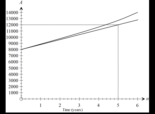
This graph compares two investments: one with simple interest (straight line) and one with compound interest (curved line). The compound interest investment grows faster over time.

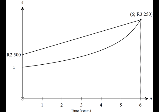
This graph shows two investments: one with simple interest starting at R2,500 and one with compound interest starting at x. Both reach R3,250 after 6 years, illustrating how a lower principal with compound interest can match a higher principal with simple interest.

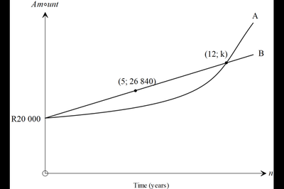
This graph compares two investments, A (compound interest) and B (simple interest), both starting at R20,000. After 12 years, investment A has grown more rapidly, demonstrating the power of compounding.

Sinking Funds

A sinking fund is a savings plan set up to accumulate a specific amount in the future, often to replace equipment or repay a debt. The required future value is calculated by considering both the depreciated value of the old asset and the inflated cost of the new asset.

• Future Value Formula: (for regular payments)

• Depreciation and Inflation: Use compound interest and reducing-balance formulas to find future and scrap values.

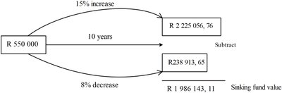
This diagram summarizes the calculation of a sinking fund value by considering the future inflated cost of new equipment and the depreciated value of the old equipment.

Summary Table: Key Financial Mathematics Formulas