15-18. {Use of Tech} Midpoint Rule approximations. Find the indicated Midpoint Rule approximations to the following integrals.
18. ∫(0 to 1) e⁻ˣ dx using n = 8 subintervals

검증된 단계별 안내

Step 1: Understand the Midpoint Rule. The Midpoint Rule is a numerical method to approximate the value of a definite integral. It divides the interval into 'n' subintervals, calculates the midpoint of each subinterval, evaluates the function at these midpoints, and sums the results multiplied by the width of the subintervals.

Step 2: Identify the interval and the number of subintervals. The integral is ∫(0 to 1) e⁻ˣ dx, and the interval is [0, 1]. The number of subintervals is n = 8.

Step 3: Calculate the width of each subinterval (Δx). The width is given by Δx = (b - a) / n, where 'a' is the lower limit and 'b' is the upper limit of the integral. Substituting the values, Δx = (1 - 0) / 8.

Step 4: Determine the midpoints of each subinterval. The midpoints are calculated as xᵢ = a + (i - 0.5)Δx for i = 1, 2, ..., n. Substitute the values of 'a' and Δx to find the midpoints for each subinterval.

Step 5: Apply the Midpoint Rule formula. The approximation is given by M₈ = Δx * Σ(f(xᵢ)), where f(x) = e⁻ˣ and xᵢ are the midpoints calculated in Step 4. Evaluate f(xᵢ) for each midpoint and sum the results, then multiply by Δx to get the approximation.

비슷한 문제에 대한 검증된 영상 답변:

이 영상 해법은 위 문제에 도움이 된다고 튜터들이 추천한 것입니다.

영상 길이:

도움이 되었나요?

주요 개념

질문에 올바르게 답하기 위해 반드시 이해해야 하는 핵심 개념들은 다음과 같습니다.

Midpoint Rule

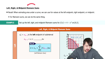
The Midpoint Rule is a numerical method used to approximate the value of a definite integral. It involves dividing the interval of integration into 'n' subintervals of equal width and using the midpoint of each subinterval to calculate the area of rectangles that approximate the area under the curve. The formula for the Midpoint Rule is given by: M_n = Δx * Σ f(x_i*), where Δx is the width of each subinterval and x_i* is the midpoint of the i-th subinterval.

Definite Integral

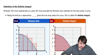
A definite integral represents the signed area under a curve defined by a function over a specific interval [a, b]. It is denoted as ∫(a to b) f(x) dx and can be interpreted as the limit of Riemann sums as the number of subintervals approaches infinity. The definite integral provides a way to calculate total accumulation, such as distance, area, or volume, depending on the context of the function.

Subintervals

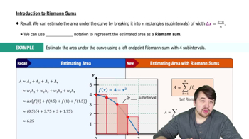
Subintervals are smaller segments into which the main interval of integration is divided when applying numerical methods like the Midpoint Rule. The number of subintervals, denoted as 'n', determines the accuracy of the approximation; more subintervals generally lead to a better approximation of the integral. The width of each subinterval is calculated as Δx = (b - a) / n, where [a, b] is the interval of integration.

15-18. {Use of Tech} Midpoint Rule approximations. Find the indicated Midpoint Rule approximations to the following integrals.18. ∫(0 to 1) e⁻ˣ dx using n = 8 subintervals