Ch. 9 - Differential Equations
Briggs - Calculus: Early Transcendentals 3rd Edition
Briggs3rd EditionCalculus: Early TranscendentalsISBN: 9780136847243당신이 사용하는 게 아니라요?교과서 변경
9장, 문제 9.5.21

20–22. {Use of Tech} Solving the Gompertz equation Solve the Gompertz equation in Exercise 19 with the given values of r, K, and M₀. Then graph the solution to be sure that M(0) and lim(t→∞) M(t) are correct.


r = 0.05, K = 1200, M₀ = 90

검증된 단계별 안내
1
Recall the Gompertz differential equation, which is commonly written as \(\frac{dM}{dt} = r M \ln\left(\frac{K}{M}\right)\), where \(M(t)\) is the population at time \(t\), \(r\) is the growth rate, and \(K\) is the carrying capacity.
To solve this equation, start by separating variables or using an integrating factor approach. The general solution to the Gompertz equation can be expressed as \(M(t) = K \exp\left(-C e^{-r t}\right)\), where \(C\) is a constant determined by the initial condition.
Apply the initial condition \(M(0) = M_0\) to find the constant \(C\). Substitute \(t=0\) and \(M(0) = M_0\) into the solution formula to get \(M_0 = K \exp(-C)\), which implies \(C = -\ln\left(\frac{M_0}{K}\right)\).
Substitute the value of \(C\) back into the solution to get the explicit formula for \(M(t)\): \(M(t) = K \exp\left(-\left(-\ln\left(\frac{M_0}{K}\right)\right) e^{-r t}\right)\), which simplifies to \(M(t) = K \exp\left(\ln\left(\frac{M_0}{K}\right) e^{-r t}\right)\).
Finally, use the given values \(r=0.05\), \(K=1200\), and \(M_0=90\) to write the specific solution. Then, graph \(M(t)\) over a suitable range of \(t\) to verify that \(M(0) = 90\) and that \(\lim_{t \to \infty} M(t) = K = 1200\).

비슷한 문제에 대한 검증된 영상 답변:

이 영상 해법은 위 문제에 도움이 된다고 튜터들이 추천한 것입니다.
영상 길이:
4m
도움이 되었나요?

주요 개념

질문에 올바르게 답하기 위해 반드시 이해해야 하는 핵심 개념들은 다음과 같습니다.

Gompertz Equation

The Gompertz equation is a type of differential equation used to model growth processes, often in biology or demography. It describes how a quantity grows rapidly at first and then slows down as it approaches a limiting value, called the carrying capacity. Understanding its form and parameters is essential to solving and interpreting the solution.
추천 영상:
08:02
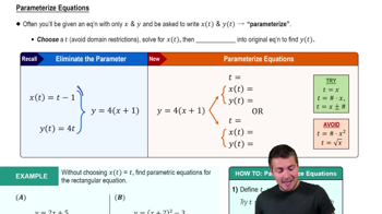
Parameterizing Equations

Initial Conditions and Parameters

Initial conditions like M₀ specify the starting value of the function at time zero, while parameters r and K control the growth rate and the upper limit (carrying capacity) respectively. Correctly applying these values is crucial for finding the particular solution that fits the given scenario.
추천 영상:
가이드 코스
05:03
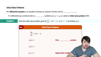
Initial Value Problems

Limit Behavior and Graphing Solutions

Analyzing the limit of M(t) as t approaches infinity helps verify the long-term behavior of the solution, ensuring it approaches the carrying capacity K. Graphing the solution visually confirms the initial value and asymptotic behavior, providing insight into the model’s accuracy and dynamics.
추천 영상:
가이드 코스
06:15
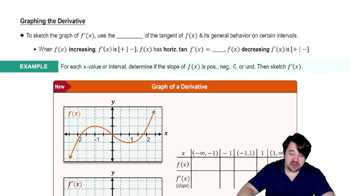
Graphing The Derivative