Chapter 6: Higher-Degree Polynomial and Rational Functions

Objectives

• Identify the degrees and leading coefficients of polynomials.

• Factor higher-degree polynomials completely.

• Simplify rational expressions.

• Multiply and divide rational expressions.

• Add and subtract rational expressions.

• Simplify complex fractions.

• Divide polynomials using long division.

Degrees and Leading Coefficients

Definition and Identification

Every polynomial function can be written in the form , where is a non-negative integer. The degree of the polynomial is the highest power of with a nonzero coefficient, and the leading coefficient is the coefficient of the term with the highest degree.

• Degree: Indicates the highest exponent in the polynomial.

• Leading Coefficient: The coefficient of the term with the highest degree.

• Example: For , the degree is 5 and the leading coefficient is 4.

Factoring Higher-Degree Polynomials

Complete Factorization

Factoring involves expressing a polynomial as a product of lower-degree polynomials. This process is essential for simplifying expressions and solving equations.

• Look for common factors first.

• Apply factoring techniques such as grouping, difference of squares, sum/difference of cubes, and quadratic form.

• Example:

Simplifying Rational Expressions

Definition and Simplification

A rational expression is a fraction in which the numerator and denominator are both polynomials. Simplifying involves factoring both and canceling common factors.

• Factor numerator and denominator completely.

• Divide out any common factors.

• Example: ,

Multiplying and Dividing Rational Expressions

Procedures and Examples

Multiplying and dividing rational expressions follows the same rules as with numerical fractions, with the added step of factoring polynomials.

• Multiplication: Multiply numerators together and denominators together, then simplify.

• Division: Invert the divisor and multiply.

• Example: ,

Adding and Subtracting Rational Expressions

Finding the Least Common Denominator (LCD)

To add or subtract rational expressions, first find the LCD, rewrite each expression with the LCD, combine numerators, and simplify.

• Completely factor each denominator.

• The LCD is the product of each different factor, each used the maximum number of times it occurs in any denominator.

• Rewrite each expression with the LCD, combine numerators, and simplify.

• Example:

Simplifying Complex Fractions

Step-by-Step Simplification

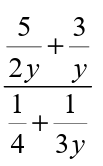
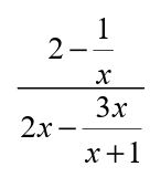
A complex fraction is a fraction in which the numerator, denominator, or both, contain fractions themselves. Simplification involves finding the LCD of all fractions in the numerator and denominator, multiplying through, and simplifying.

• Find the LCD of all fractions in the numerator and denominator.

• Multiply both numerator and denominator by the LCD.

• Simplify each term and reduce the resulting fraction if possible.

Example:

Dividing Polynomials Using Long Division

Algorithm and Example

Long division is used to divide a polynomial by another polynomial of lower or equal degree. The process is similar to numerical long division.

• Arrange both polynomials in descending powers of the variable.

• Divide the leading term of the dividend by the leading term of the divisor to get the first term of the quotient.

• Multiply the divisor by this term, subtract from the dividend, and repeat with the new polynomial.

• Continue until the degree of the remainder is less than the degree of the divisor.

• The result is written as:

Section 6.1: Higher Degree Polynomial Functions

Identifying and Graphing Higher-Degree Polynomial Functions

Polynomial functions of degree three or higher are called higher-degree polynomials. Their graphs exhibit more complex behavior, including multiple turning points and intercepts.

• The graph of a degree polynomial has at most turning points and at most x-intercepts.

• The end behavior is determined by the degree and leading coefficient.

Cubic Functions

A cubic function has the general form . Its graph typically has one or two turning points and exhibits "opposite end behavior" (one end up, one end down).

• If the leading coefficient , the right end rises; if , the right end falls.

• There can be 0 or 2 turning points (local extrema).

• The graph can have up to 3 x-intercepts.

• Local minimum: Point where the graph changes from decreasing to increasing.

• Local maximum: Point where the graph changes from increasing to decreasing.

• Absolute minimum/maximum: Lowest/highest point on a given interval.

Quartic Functions

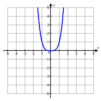
A quartic function is a fourth-degree polynomial, . The basic quartic function has a "W" or "M" shape, depending on the coefficients.

• If the leading coefficient , both ends of the graph rise to infinity.

• If , both ends fall to negative infinity.

• There can be up to 3 turning points and 4 x-intercepts.

General Properties of Polynomial Graphs

• A degree polynomial has at most turning points.

• It has at most x-intercepts.

• Odd-degree polynomials: End behavior is "one end up, one end down."

• Even-degree polynomials: End behavior is "both ends up" or "both ends down."

Examples: Analyzing Polynomial Graphs

Example 1

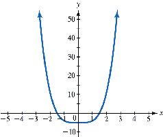
• Number of x-intercepts: Count the points where the graph crosses the x-axis.

• Number of turning points: Count the local maxima and minima.

• Leading coefficient: If the right end rises, it is positive; if it falls, it is negative.

• Degree: Odd if ends go in opposite directions; even if both ends go the same way.

• Minimum possible degree: One more than the number of turning points.

Example 2

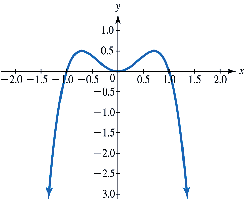
• Repeat the analysis as above for this graph.

Example 3

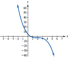
• Repeat the analysis as above for this graph.

Example 4

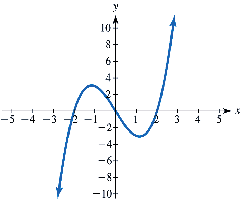
• Repeat the analysis as above for this graph.

Additional info: For each graph, students should practice identifying the number of x-intercepts, turning points, the sign of the leading coefficient, whether the degree is odd or even, and the minimum possible degree based on the graph's features.