Sect 4.1: Linear Functions

Definition and Properties of Linear Functions

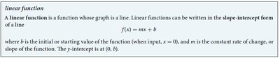
Linear functions are fundamental in algebra, representing relationships where the rate of change is constant. The graph of a linear function is always a straight line, and it can be written in the slope-intercept form:

• Slope-Intercept Form:

• b: The initial or starting value of the function (when input, )

• m: The constant rate of change, or slope of the function

• y-intercept: The point where the line crosses the y-axis

Increasing, Decreasing, and Constant Linear Functions

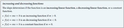
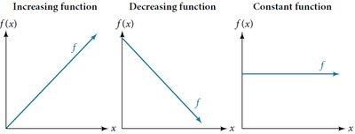
The slope () determines whether a linear function is increasing, decreasing, or constant:

• Increasing Function: is increasing if

• Decreasing Function: is decreasing if

• Constant Function: is constant if

Calculating Slope and Rate of Change

The slope or rate of change of a linear function is calculated using two points and :

• Slope Formula:

• This formula measures how much changes for each unit change in .

Example: If Molly has $1700 initially and $1130 after 6 months, the rate of change is:

• This means Molly spends $95 per month.

Modeling Real-World Situations with Linear Functions

Linear functions are used to model various real-world scenarios, such as population growth, costs, and yields.

• Cost Function Example: If Ben incurs a fixed cost of C(x) = 37.5x + 1250$.

• Yield Example: If a farmer plants 4 stalks yielding 120 ounces and 9 stalks yielding 220 ounces, the slope is . The linear function is (solve for using one of the points).

Graphing Linear Functions

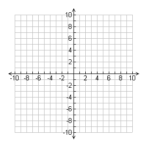
To graph a linear function, plot the y-intercept and use the slope to determine the direction and steepness of the line.

• Start at

• From the y-intercept, move up/down by the slope for each unit right

Sect 4.2: Modeling with Linear Functions

Constructing Linear Models

Linear models are used to describe relationships where the rate of change is constant. The general form is .

• Airplane Descent Example: If an airplane starts at 35,000 feet and descends at 1,200 feet per minute, the model is .

• Piecewise Linear Example: A recycling center pays A(x) = 20 + 0.15xx > 0$.

• Magazine Circulation Example: If circulation grows from 1 million in 2004 to 2 million in 2014, the slope is million per year. The model is where is years after 2004.

Solving Linear Equations Analytically and Graphically

To find when two linear functions are equal, set their equations equal and solve for the variable. Graphically, plot both lines and find the intersection.

• Example: Two cars with different starting gas volumes and rates of consumption. Set and solve for .

• For cost comparisons (e.g., ice rinks), set and solve for (hours).

Sect 4.3: Fitting Linear Models to Data

Scatter Plots and Linear Relationships

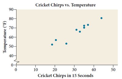
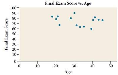
A scatter plot is a graph of points representing paired data. It helps visualize whether a linear relationship exists between two variables.

• Trend Example: As cricket chirps increase, temperature increases, suggesting a positive linear relationship.

• No Trend Example: Final exam scores vs. age show no clear trend.

Correlation Coefficient

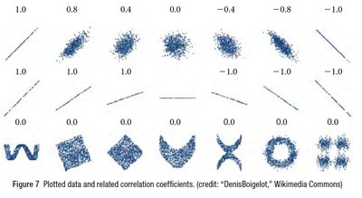
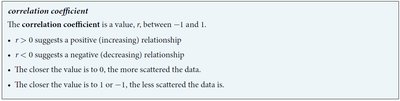
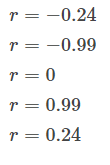
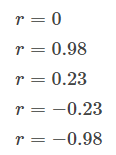
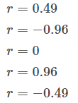
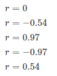
The correlation coefficient () measures the strength and direction of a linear relationship between two variables. It ranges from -1 to 1.

• : Positive (increasing) relationship

• : Negative (decreasing) relationship

• The closer is to 1 or -1, the stronger the linear relationship

• The closer is to 0, the weaker the relationship

Estimating Correlation Coefficient from Plots

Given a scatter plot, estimate by observing the direction and tightness of the data points.

• Strong positive trend: close to 1

• Strong negative trend: close to -1

• No trend: close to 0

Finding Linear Regression Equations

Linear regression finds the best-fit line for a set of data points. The equation is typically , where and are determined by minimizing the sum of squared errors.

• Use a graphing calculator to input data, create a scatter plot, and calculate the regression equation.

• Steps for TI-83/84 calculators:

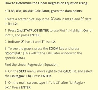
• Sketch the scatter plot

• Check if the data fits a linear trend

• Find the regression equation and use it for predictions

Applications of Linear Regression

Once the regression equation is found, it can be used to estimate values, analyze trends, and make predictions for new data points.

• Example: Using the regression equation, find when .