Polynomial Functions and Their Graphs

Definition of a Polynomial Function

A polynomial function is a function of the form:

where n is a nonnegative integer, and the coefficients are real numbers with . The highest power of x (n) is called the degree of the polynomial, and is the leading coefficient.

Graphs of Polynomial Functions: Smoothness and Continuity

Polynomial functions of degree 2 or higher have graphs that are smooth (no sharp corners) and continuous (no breaks; can be drawn without lifting your pencil).

End Behavior of Polynomial Functions

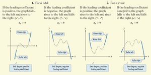
The end behavior of a polynomial function describes how the graph behaves as approaches or . This behavior is determined by the degree and the leading coefficient of the polynomial.

The Leading Coefficient Test

The Leading Coefficient Test helps predict the end behavior of a polynomial function:

• If the degree is even and the leading coefficient is positive, the graph rises to both the left and right.

• If the degree is even and the leading coefficient is negative, the graph falls to both the left and right.

• If the degree is odd and the leading coefficient is positive, the graph falls to the left and rises to the right.

• If the degree is odd and the leading coefficient is negative, the graph rises to the left and falls to the right.

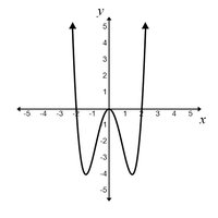
Example: Using the Leading Coefficient Test

Consider . The degree is 4 (even), and the leading coefficient is 1 (positive). Thus, the graph rises to the left and right.

Zeros of Polynomial Functions

The zeros of a polynomial function are the values of for which . These are also called roots or solutions of the equation . Each real zero corresponds to an x-intercept of the graph.

Example: Finding Zeros

Find all zeros of :

Set :

So, and are zeros.

Multiplicity and x-Intercepts

If a zero of a polynomial has multiplicity (i.e., is a factor):

• If is even, the graph touches the x-axis at and turns around.

• If is odd, the graph crosses the x-axis at .

• For , the graph flattens out near .

Example: Finding Zeros and Their Multiplicities

For :

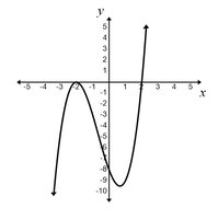
• is a zero of multiplicity 2 (even): graph touches and turns at .

• is a zero of multiplicity 1 (odd): graph crosses at .

The Intermediate Value Theorem

The Intermediate Value Theorem states: If is a polynomial function with real coefficients, and and have opposite signs, then there is at least one value between and such that . This means there is at least one real root between and .

Example: Using the Intermediate Value Theorem

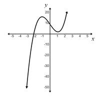
For , and . Since the signs are opposite, there is a real zero between and .

Turning Points of Polynomial Functions

A turning point is a point where the graph changes direction from increasing to decreasing or vice versa. For a polynomial of degree , the graph has at most turning points.

A Strategy for Graphing Polynomial Functions

To graph a polynomial function, follow these steps:

1. Determine end behavior using the Leading Coefficient Test.

2. Find x-intercepts (zeros) by solving . Note the multiplicity of each zero.

3. Find the y-intercept by computing .

4. Check for symmetry:

   • y-axis symmetry: (even function)

   • Origin symmetry: (odd function)

5. Check the number of turning points (should not exceed ).

Example: Graphing a Polynomial Function

Let .

• Step 1: End behavior – degree 3 (odd), leading coefficient 2 (positive): falls left, rises right.

• Step 2: x-intercepts – (multiplicity 2), (multiplicity 1).

• Step 3: y-intercept – .

• Step 4: Symmetry – neither y-axis nor origin symmetry.

• Step 5: Turning points – maximum is ; graph has two turning points.

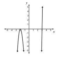
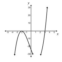
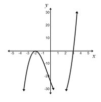
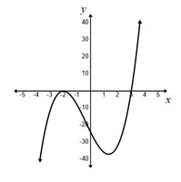
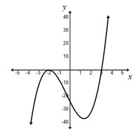
Additional info: The above strategy ensures a systematic approach to sketching polynomial graphs, emphasizing the importance of intercepts, end behavior, and turning points for accurate representation.