뒤로
뒤로Aqueous Ionic Equilibrium: Buffers, Titrations, and Solubility
스터디 가이드 - 스마트 노트
 자료에 맞춘 맞춤형 노트, 핵심 정의, 예시, 맥락을 확장해 제공합니다.
Aqueous Ionic Equilibrium
Acid-Base Buffers
Acid-base buffers are solutions that resist drastic changes in pH when small amounts of acid or base are added. Buffers contain both a weak acid and its conjugate base, or a weak base and its conjugate acid, which neutralize added H+ and OH- ions, respectively.
Key Point 1: Buffers are made from a weak acid and its conjugate base, or a weak base and its conjugate acid.
Key Point 2: Buffers neutralize added acids and bases, maintaining pH stability.
Example: A mixture of acetic acid (CH3COOH) and sodium acetate (CH3COONa) forms a buffer.
Buffer Capacity and Range
Buffer capacity is the amount of acid or base a buffer can neutralize before the pH changes significantly. The higher the concentration of buffer components, the greater the buffer capacity. The buffer range is the pH range over which the buffer is effective, typically when the ratio of weak acid to conjugate base is between 1:10 and 10:1.
Key Point 1: Buffer capacity increases with higher concentrations of buffer components.
Key Point 2: Buffer is most effective when [weak acid] = [conjugate base].
Example: A buffer with 0.5 M acetic acid and 0.5 M sodium acetate has high capacity and is effective near pH = pKa of acetic acid.
Henderson-Hasselbalch Equation
The Henderson-Hasselbalch equation allows calculation of the pH of a buffer solution without using an ICE chart. It applies to buffers composed of weak acid-base pairs.
Key Point 1: The equation relates pH, pKa, and the ratio of conjugate base to weak acid.
Key Point 2: For a weak acid buffer:
Example: Calculate the pH of a solution containing 2.0 M HNO2 and 1.48 M LiNO2 (Ka = 4.6 x 10⁻⁴):
Acid-Base Titration Curves
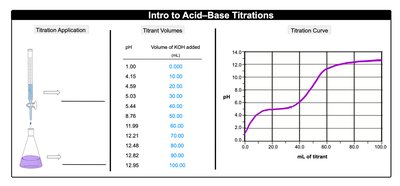
An acid–base titration is a reaction used to determine the concentration of an acid or base. The titration curve is a graph of the pH of the titrate during the titration with a titrant. The equivalence point is where the moles of acid equal the moles of base.
Key Point 1: The equivalence point is the steepest region of the titration curve.
Key Point 2: For strong acid–strong base titrations, the pH at equivalence is 7.0.
Example: Titration of 40.0 mL of 0.0550 M H2CO3 with 0.160 M Al(OH)3 requires calculation of volumes using .
Strong Titrate–Strong Titrant Curves
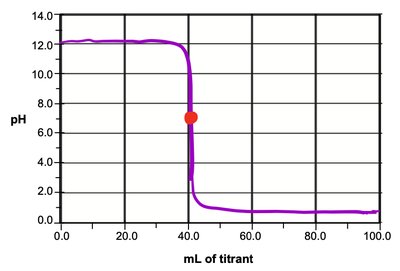
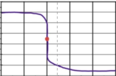
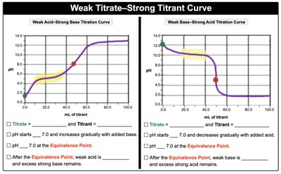
When both titrate and titrant are strong acids or bases, the titration curve shows a sharp change in pH at the equivalence point. The pH starts below 7.0 for strong acid titrate and above 7.0 for strong base titrate.
Key Point 1: pH at equivalence point is 7.0 for strong acid–strong base titrations.
Key Point 2: After equivalence, excess titrant determines the pH.
Weak Titrate–Strong Titrant Curves
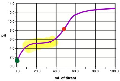
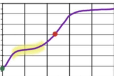
For titrations involving a weak acid or base and a strong titrant, the curve has a buffer region where pH changes gradually. The half equivalence point is where [weak acid] = [conjugate base], and pH = pKa.
Key Point 1: Buffer region is where pH is most resistant to change.
Key Point 2: At half equivalence, pH = pKa.
Example: Titration of 30.0 mL of 0.100 M HC2H3O2 with 0.100 M NaNH2 shows buffer region before equivalence.
Acid-Base Indicators
Acid-base indicators are weak acids or bases that change color at a specific pH range, marking the endpoint of a titration. The best indicator for a titration is one whose pKa is close to the pH at the equivalence point.
Key Point 1: Indicators change color when the ratio of [weak form] to [conjugate form] shifts.
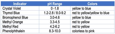
Key Point 2: Each indicator has a characteristic pH range and color change.
Indicator | pH Range | Colors |
|---|---|---|
Crystal Violet | 0 - 1.8 | yellow to blue |
Thymol Blue | 1.2-2.8 / 8.0-9.2 | red to yellow/yellow to blue |
Bromophenol Blue | 3.0-4.6 | yellow to blue |
Methyl Orange | 3.3-4.5 | red to yellow |
Methyl Red | 4.2-6.2 | red to yellow |
Phenolphthalein | 8.3-10.0 | colorless to pink |
Titrations: Weak Acid–Strong Base
In titrations where a weak acid is titrated with a strong base, an ICF (Initial, Change, Final) chart is used to calculate the amounts of compounds. Before the equivalence point, the strong base neutralizes the weak acid, forming conjugate base.
Key Point 1: Use the Henderson-Hasselbalch equation to find pH in the buffer region.
Key Point 2: At equivalence, only conjugate base remains; use ICE chart to solve for pH.
Titrations: Weak Base–Strong Acid
When a weak base is titrated with a strong acid, similar steps are followed. Before equivalence, the strong acid neutralizes the weak base, forming conjugate acid.
Key Point 1: Use the Henderson-Hasselbalch equation for pH in the buffer region.
Key Point 2: At equivalence, only weak acid (conjugate acid) remains; use ICE chart to solve for pH.
Titrations: Strong Acid–Strong Base
For titrations involving strong acids and strong bases, use an ICF chart to determine the concentration of the remaining strong species. The pH is calculated directly from [H+] or [OH-].
Key Point 1: At equivalence, pH = 7.0.
Key Point 2: After equivalence, excess strong acid or base determines pH.
Diprotic and Polyprotic Buffers
Diprotic and polyprotic acids have multiple equivalence points and require multiple Henderson-Hasselbalch equations due to multiple Ka values. The relationships between equivalence points and equations are important for calculating pH during titration.
Key Point 1: Each dissociation step has its own pKa and buffer region.
Key Point 2: Use appropriate Henderson-Hasselbalch equation for each region.
Solubility Product Constant: Ksp
The solubility product constant (Ksp) measures the solubility of solid ionic compounds in a solvent at equilibrium. Solubility is the maximum amount of solid dissolved, usually represented as molar solubility (M).
Key Point 1: Higher Ksp means more soluble; lower Ksp means less soluble.
Key Point 2: Ksp calculations require ICE charts and equilibrium expressions.
Example: For PbF2:
Ksp: Common Ion Effect
The common ion effect decreases the solubility of a solid in a solution containing ions common to the solid. This is explained by Le Chatelier’s principle.
Key Point 1: Solubility decreases in the presence of a common ion.
Key Point 2: Use ICE charts to calculate new solubility.
Precipitation: Ksp vs Q
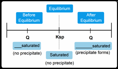
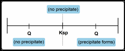
Ksp helps determine how soluble an ionic solid can be at equilibrium. Q (reaction quotient) is compared to Ksp to predict whether a precipitate will form.
Key Point 1: If Q < Ksp, solution is unsaturated (no precipitate).
Key Point 2: If Q > Ksp, solution is supersaturated (precipitate forms).
Selective Precipitation
Selective precipitation separates specific ions from a solution by using reagents that form a precipitate with the ions. The success depends on the Ksp of the salt.
Key Point 1: Precipitation occurs when Q > Ksp for a specific ion.
Key Point 2: Use Ksp values to determine which ion will precipitate first.
Complex Ions: Formation Constant
A complex ion contains a metal cation (Lewis acid) covalently bonded to a ligand (Lewis base). The formation constant (Kf) is the equilibrium constant for the formation of complex ions.
Key Point 1: Kf is calculated using equilibrium expressions for complex ion formation.
Key Point 2: ICE charts are used to determine concentrations at equilibrium.
Example: Ag+ + 2 CN- ⇌ Ag(CN)2-, Kf = 1.0 x 10²¹
Mathematical Operations in Chemistry
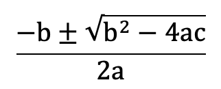
Many equilibrium and titration calculations require solving quadratic equations. The quadratic formula is used to solve for unknown concentrations.
Key Point 1: Quadratic formula: