The Solow Growth Model

Introduction to the Steady State

The Solow Growth Model is a foundational framework in macroeconomics for understanding long-run economic growth, capital accumulation, and differences in income across countries. The model focuses on how savings, investment, and depreciation interact to determine the steady state of an economy.

• Steady State: The point at which capital per worker, output per worker, and consumption per worker remain constant over time.

• Capital Law of Motion: Describes how capital evolves: , where is investment and is depreciation.

• At steady state: , so .

Solving for the Steady State

To find the steady state, set investment equal to depreciation and solve for the steady-state capital stock:

• Production Function (per worker):

• Steady-State Output:

• Steady-State Capital:

• Where is the savings rate, is the depreciation rate, is the population growth rate, and is total factor productivity (TFP).

Comparative Statics and Parameter Changes

The steady-state values depend on key parameters:

• Increase in Savings Rate (): Raises steady-state capital and output per worker.

• Increase in Depreciation Rate (): Lowers steady-state capital and output per worker.

• Increase in Productivity (): Raises steady-state capital and output per worker.

• Population Growth (): Higher reduces steady-state capital per worker and output per worker.

Transition Dynamics

Transition dynamics describe how an economy moves from one steady state to another after a change in parameters (e.g., savings rate, productivity, depreciation rate):

• If the economy is below its steady state, it will grow rapidly; if above, it will contract.

• The further from steady state, the faster the adjustment; as the steady state is approached, growth slows to zero.

Empirical Evidence: Growth Rates and Transition Dynamics

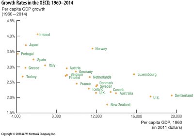
Empirical data supports the principle of transition dynamics, especially among OECD countries. Poorer countries in 1960 grew faster than richer ones, consistent with the Solow model's predictions.

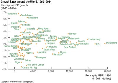
However, when examining the world as a whole, the relationship is less clear, suggesting that differences in parameters (such as savings rates and productivity) also play a significant role.

Case Study: South Korea and the Philippines

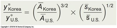
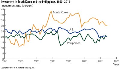
Comparing South Korea and the Philippines illustrates the impact of investment rates and productivity on long-run income levels. South Korea's rapid growth is explained by its position far below steady state in 1960 and its high investment rate, while the Philippines remained near its steady state with lower investment.

• Long-run per capita income ratio:

• Investment rates over time: South Korea's investment rate was consistently higher than that of the Philippines and the U.S., supporting its rapid growth.

Economic Growth in the Solow Model

The Solow model predicts that in the long run (steady state), there is no growth in output per worker or capital per worker—these variables become constant. However, in reality, economies often continue to grow, highlighting a limitation of the model: it does not explain sustained long-run growth, which is often attributed to technological progress (TFP growth).

• Population Growth: Increases aggregate output but not output per worker due to diminishing returns.

• Capital Accumulation: Drives growth only in the transition to steady state, not in the long run.

Strengths and Weaknesses of the Solow Model

• Strengths:

  • Explains differences in income levels across countries.

  • Provides a framework for understanding transition dynamics and the impact of savings, investment, and depreciation.

• Weaknesses:

  • Does not explain the source of long-run growth (TFP is exogenous).

  • Does not endogenize the savings/investment rate.

  • Cannot explain persistent differences in growth rates without appealing to differences in parameters.

Solow Diagram and Transition Dynamics

The Solow diagram visually represents the relationship between investment, depreciation, and capital stock. The intersection of the investment and depreciation curves determines the steady-state capital stock (). If the economy starts below $K^*$, capital accumulates; if above, capital declines, always converging to $K^*$.

• Key Principle: Regardless of starting point, the economy transitions toward the steady state.

Summary Table: Effects of Parameter Changes on Steady State

Additional info: The Solow model is a cornerstone of macroeconomic growth theory, but modern research often extends it by endogenizing technological progress (e.g., endogenous growth models) to explain sustained long-run growth.