Trade and Comparative Advantage

Production Possibilities and the Basis for Trade

The production possibilities curve (PPC) illustrates the maximum output combinations of goods or services that can be produced with available resources and technology. The foundation of trade between individuals or nations is comparative advantage, which refers to the ability to produce a good at a lower opportunity cost than others. Specialization and trade allow for increased total output, as each agent focuses on goods where they have comparative advantage.

• Comparative Advantage: Producing at lower opportunity cost than another agent.

• Absolute Advantage: Producing more output with the same resources than another agent.

• Specialization: Agents specialize in goods where they have comparative advantage, increasing total production.

• Winners and Losers: Trade creates winners and losers, but overall gains can compensate losses.

• Arguments Against Free Trade: Include concerns about job losses, national security, and unfair competition.

Example: If you can produce computer programs at a lower opportunity cost than Olivia, and Olivia can produce websites at a lower opportunity cost than you, specialization and trade will increase total output.

Externalities and Public Goods

Public Goods and Common Pool Resources

Public goods are non-rival and non-excludable, meaning one person's consumption does not reduce availability for others, and it is difficult to prevent anyone from using them. Examples include national defense and bridges. The main issue with public goods is under-provision due to the free rider problem, where individuals benefit without paying.

• Non-Excludable: Cannot prevent people from using the good.

• Non-Rival: One person's use does not diminish another's.

• Free Rider Problem: Individuals avoid paying, leading to under-investment.

• Government Solutions: Mandatory payment or provision to address under-investment.

Externalities

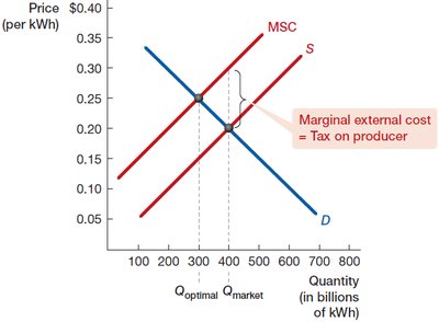
Externalities are spillover effects from economic activities that affect third parties. Negative externalities (e.g., pollution) impose costs, while positive externalities (e.g., education) provide benefits. Private solutions include bargaining (Coase Theorem), while government solutions include corrective taxes (Pigouvian taxes).

• Negative Externality: Activity imposes costs on others.

• Positive Externality: Activity provides benefits to others.

• Pigouvian Tax: Tax equal to marginal external cost to incentivize optimal output.

Markets for Factors of Production

Labor Markets

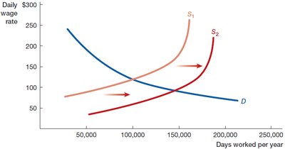
Labor is a key factor of production. Firms demand labor based on the value of the marginal product of labor (VMPL), while workers supply labor by trading off earnings against foregone leisure. Wage inequality arises from differences in human capital, compensating wage differentials, and discrimination.

• Factors of Production: Labor, physical capital, land.

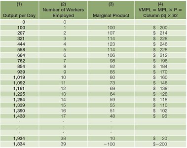
• VMPL: Value of Marginal Product of Labor = Marginal Product × Price.

• Labor Supply: Determined by opportunity cost of leisure.

• Wage Inequality: Human capital, compensating differentials, discrimination.

Labor Demand and Supply Curves

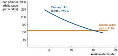
The demand for labor is downward sloping, reflecting diminishing marginal returns. Firms hire workers up to the point where VMPL equals the wage rate. Labor supply can shift due to population changes, preferences, and opportunity costs.

• Profit Maximization: Hire workers until VMPL = Wage.

• Labor Supply Shifts: Population, preferences, opportunity costs.

Monopoly

Monopoly Market Structure

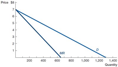
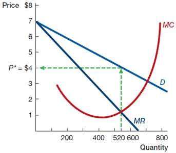
A monopoly is a market with a single seller and no close substitutes. Monopolists are price makers, setting prices above marginal cost and producing less than perfectly competitive firms, resulting in deadweight loss. Efficiency can be improved through price discrimination or government intervention.

• Monopoly: One seller, barriers to entry.

• Profit Maximization: Produce where MR = MC.

• Deadweight Loss: Monopoly reduces total surplus compared to perfect competition.

• Price Discrimination: Charging different prices to different consumers to increase efficiency.

Equations:

• For a straight-line demand curve:

• Marginal Revenue:

• Profit:

Game Theory and Strategic Play

Elements of a Game and Nash Equilibrium

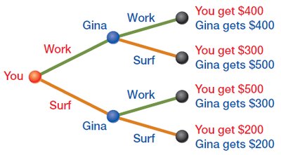
Game theory analyzes strategic interactions among players. Each player chooses strategies to maximize payoffs. A Nash equilibrium occurs when no player can benefit by changing strategies, given the strategies of others. Dominant strategies are best responses regardless of others' actions.

• Players: Decision-makers in the game.

• Strategies: Possible actions for each player.

• Payoffs: Outcomes associated with strategies.

• Nash Equilibrium: No player can improve payoff by changing strategy unilaterally.

• Dominant Strategy: Best response regardless of others' actions.

Example: Prisoners' Dilemma—players choose to confess or not, payoffs depend on both choices.

Oligopoly and Monopolistic Competition

Market Structures Between Perfect Competition and Monopoly

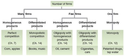
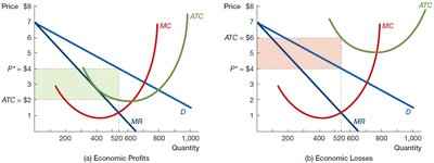
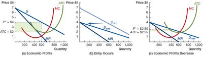
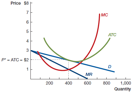
Oligopoly and monopolistic competition are intermediate market structures. Oligopolies have few firms and may earn long-run profits, while monopolistic competitors sell differentiated products and long-run profits are driven to zero by entry and exit.

• Oligopoly: Few firms, possible collusion, positive long-run profits.

• Monopolistic Competition: Many firms, differentiated products, zero long-run profits.

• Key Variables: Number of firms, product differentiation, entry barriers, collusion.

Trade-offs Involving Time and Risk

Time Value of Money

To compare present and future values, economists use the concept of the time value of money. The future value of an investment is calculated using compound interest. The Rule of 72 estimates the time required for an investment to double.

• Principal: Original investment amount.

• Interest: Payment for use of money.

• Compound Interest Formula:

• Rule of 72: Years to double = 72 / annual growth rate (%)

Time Preferences and Discounting

Individuals discount future utility, preferring immediate rewards. The discount weight translates future utility into present terms. Behavioral examples include choices between immediate and delayed rewards, such as dieting or saving.

• Utils: Measure of utility or happiness.

• Discount Weight: Multiplies future utils to convert to present utils.

Probability and Risk

Risk involves uncertain outcomes. Expected value is the probability-weighted average of possible outcomes. Present and future values are weighted by time, while expected values are weighted by probability.

• Risk: Outcome not known with certainty.

• Probability: Frequency of occurrence.

• Expected Value Formula:

Example: In a roulette game, expected value is calculated by summing payoffs multiplied by their probabilities.

Additional info: Academic context and explanations have been expanded for completeness and clarity. Tables and images included only when directly relevant to the topic.